Cold Junction Compensation: Not So Mysterious
Once you understand how differential voltages develop in response to thermal gradients along thermocouple wires, as discussed in Martin Rowe's article "Thermocouples: Simple but misunderstood" [ EDN Design center: http://www.edn.com/design/test-and-measurement/4423409/Simple--but-misunderstood ] it is possible to understand how the otherwise-mysterious, ill-named Cold Junction Compensation technique works — allowing thermocouples to measure temperatures without the cold and without the junction.
The usual practice is to leave the cold junction terminals of a thermocouple unjoined, and measure the differential voltage there, after the temperature profile stabilizes between the conjoined hot junction end, the point where temperature is to be measured, and cold junction end, that provides the temperature reference. But there are two difficulties. First, the temperature measurement is differential, and the reference temperature must be accurately known. Second, the developed differential voltage is slightly nonlinear and depends to a certain amount on which absolute temperature is used as a reference. The nonlinear effects are not large, but certainly enough to ruin the accuracy of temperature measurements. The difficulties are minimized by standardizing on one cold junction reference temperature, and then the response characteristic is consistently relative to that.
The standard reference temperature chosen for thermocouples must be relatively easy to produce — you just need a reliable source of very pure distilled water, appropriate refrigeration equipment, and a controlled environment in which you can maintain a bath with ice and water in thermal equilibrium at one atmosphere pressure. That produces a reference temperature extremely close to zero-degrees Centigrade.
Well, that kind of solution does give you the best possible measurements, but the degree of inconvenience is extraordinary. As you probably know, most thermocouple measurements do not use an ice bath for the reference temperature. The cold junction terminals are allowed to stabilize at the ambient temperature, whatever that happens to be, and then a compensation is applied to interpret the measured results — a technique known for better or worse as cold junction compensation. This introduces a small error, typically small enough to be considered an excellent trade-off for vastly improved ease-of-use.
So how is this done? You need two more important
piece of information. The first is a standard thermocouple response
curve, in tabulated or formula representation. You can find
standardized response curves at the NIST ITS-90
Thermocouple Database site
[ http://srdata.nist.gov/its90/main/its90_main_page.html
]
and elsewhere. These curves define the expected potential response
for a variety of common thermocouple materials, for each level of
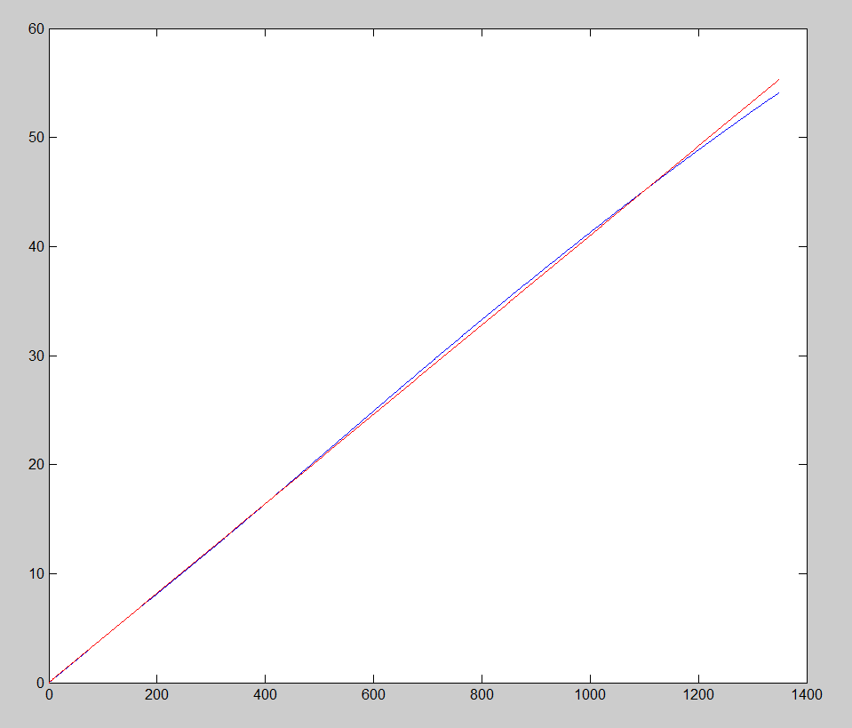
differential temperature. Here is a plot of the standardized response
curve for the popular type K thermocouple (using chromel and alumel
alloys).
Figure 1: Type K thermocouple, mV vs.
degrees C, just a little nonlinear
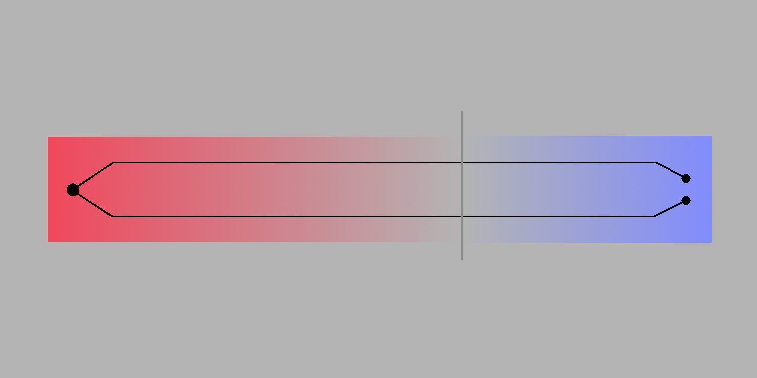
Suppose that the thermocouple measurement junction is at a high temperature, with the reference terminals in an ice bath at 0 degrees. Somewhere along the thermocouple wires, there is a location where the temperature of the wires passes the ambient temperature. Part of the total voltage differential will be developed between the hot junction point, to be measured, and the ambient temperature point. The rest will be developed between the ambient temperature point and the 0 degree reference bath.
Figure 2: Thermocouple with temperature gradient all the way to reference 0 degrees
Let us now consider what happens if we snip the thermocouple wires at the point where the temperature matches the ambient temperature. As long as the same equilibrium temperatures are maintained, the same thermal gradients and the same differential potentials exist. This it true on each side of the break. An accurate, high-impedance, differential measurement of the voltage at the ambient temperature thermocouple terminals can be measured on the hot side of the break using balanced high-conductivity leads.
Figure 3: Thermocouple with potentials above and below break at ambient temperature
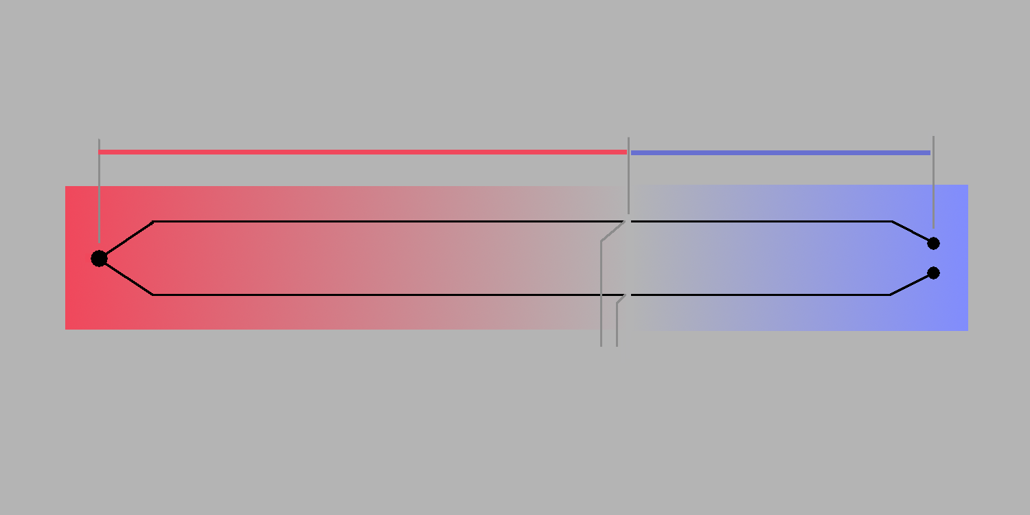
The temperature difference from ambient to cold junction is not very big, and neither is the corresponding potential. We can predict this part of the differential voltage using the second extra piece of information, a relatively accurate direct measurement of ambient temperature, obtained using a temperature sensor specialized for this purpose.
The standard thermocouple response curve can be applied to determine the potential difference typically expected between the 0 degree reference and measured ambient temperature point. This prediction is not perfect, but any well-manufactured thermocouple device has little opportunity to deviate very much from the standard device response curve over this small range. By adding the measured differential potential on the “hot side” to the estimated potential from the standard response tables for the “cold side,” the total differential voltage from "hot junction" to “cold reference” is estimated with pretty good accuracy. The physical elements below ambient temperature are no longer needed and can be removed.
An immediate follow-up to this, given the total developed potential, the NIST standard curve could be applied in the inverse direction to determine the temperature difference from the hot junction point relative to the 0 degree reference. While this idea is sound, it extends the assumption that the particular thermocouple device matches published ideal device tables through the entire range of the measurement. This common assumption is more difficult to justify, and it contributes significantly to the total measurement error.
To summarize the conventional process:
-
Measure ambient temperature,
Tambient, using a separate dedicated sensor -
Apply the standard thermocouple response curve to estimate the missing reference-side potential difference,
Vcjc = F( Tambient - Treference) -
Measure the differential potential
Vmeasat the open thermocouple terminals, ambient temperature -
Calculate the total hot junction to cold junction differential response,
V = Vmeas + Vcjc -
Apply the standard response curve in the inverse direction,
F-1( Vtotal )to obtain an estimate of the hot junction temperature.
This technique works fine, as long as you understand its limitations. Every time the words "generally", "approximately", "typically", or "measured" appear, there is an associated error. Let's take into account how these errors influence the results.
* The standard curves are subject to an approximation error. This "error of estimate" is on the order of a couple hundredths of degrees C, as reported in the NIST documents. That is to say, if the rigorous techniques that NIST used to evaluate the response curves were to be repeated on another batch of carefully manufactured thermocouple devices, we can expect that the values generated for the new tables would not deviate from the values in the currently published tables by more than a few hundredths of a degree. Compared to other sources of error, this is negligible. You will not go far wrong assuming that tabulated NIST tables and corresponding curve formulas represent typical thermocouple behaviors perfectly. (Careful, this is not the same as representing every thermocouple perfectly!)
* The NIST standard tables and formulas are complicated to apply directly in an automatic manner. Clever integrated devices approximate the tables in various ways, using nonlinear device characteristics to generate the response in an electronic analog form, or using simplified formulas such as piecewise linear or polynomial curves. The approximations to the NIST tables typically contribute errors of 0.1 degrees for each forward or reverse table evaluation.
* An absolute ambient temperature measurement can be obtained using thermistor or semiconductor sensors specialized for this purpose. Specialized "thermocouple measurement amplifier" devices are likely to include a semiconductor temperature reference circuit on-chip. These sensors can produce quite good accuracy for quite low cost, but are not perfect, typically contributing 0.1 to 0.5 degrees C to the net error, depending on the tolerances of the sensor device.
* The ambient temperature sensor measures the temperature at the sensor, which is not necessarily exactly the same as the ambient temperature at the thermocouple terminals, particularly when there is a physical separation. Any temperature displacement is reflected directly in the final measurement error.
* Attaching a differential measurement instrument at the ambient measurement terminals introduces additional junctions of dissimilar metals, possibly with stray thermocouple effects. With balanced differential signal leads, and thermal equilibrium at the ambient temperature, the stray thermocouple effects should be minimal, but there is a possibility of small residual errors.
* Manufacturers of thermocouple wires will strive to alloy materials to match the standard curves as closely as possible, but this is never perfect. Following manufacture, various subtle effects such as mechanical damage from spooling the thermocouple wire, moisture, oxidation, or minor chemical contamination, can cause variations in charge mobility and thus contribute additional small errors. It doesn't take a huge effect to be observable in measurements, since the thermocouple potential is very small. Individual device variations typically result in measurement errors in the range 1 to 2 degrees C, depending on the device type and grade.
* Thermocouples are noisy! Extremely so. The Seebeck Effect thermal response and quantum thermal noise effects are at roughly the same level. The measurements can be cleaned up a lot by filtering and averaging — but some residual measurement noise always remains. Filtering introduces a time lag, and that can add a tracking error for temperatures that are changing.
Perhaps the main thing to understand is that the principle of "garbage in garbage out" applies as much to measurements as it does to software. You can't take a thermocouple device rated plus or minus 2 degrees C, apply NIST standard curves rated plus or minus 0.02 degrees C, and expect measurements that are accurate to plus or minus 0.02 degrees C. You can't apply a high-quality integrated measurement device approximating the NIST curves with less than 0.01 percent error, supply a measurement with combined errors of more than 0.5 percent, and expect results with under 0.01 percent error.
Clearly the largest source of error is the variations in the individual thermocouple sensors. There is no way that standardized device response curves can predict what these variations will be. You can eliminate a large portion of the total measurement error by individually calibrating your thermocouples. When doing so, you can either use standard curves for calculating cold junction compensation voltages, accepting the relatively small errors that the approximation introduces, or you can independently calibrate the cold junction compensation response for each sensor.