Verifying the Model

Last time, parameters determined by a Least Squares analysis were recast from an ARMA model into the form of a dynamic state transition model using a matrix shift register construct. However, we mentioned that the new model will face some different conditions when it is applied. Specifically, the Least Squares fit has full information about what the "real system" outputs are, but this information is not available to the model as it runs. The best the model can do is substitute its prior predicted outputs for the actual output history. Using estimates in place of real values is bound to have some consequences.

New errors introduced at each step are likely to be small, initiated by small random influences. However, once an error affects one of the state variables, that influence can spread to more state variables, and like Ray Bradbury's butterfly effect,^[1] eventually can produce a much larger deviation. Just how much larger? One way to find out is to apply some data to the model, and see what happens.

 

Simulation Configuration

The model establishes values for the following matrices, as set up in the previous installment.

• Matrix Amat - The state transition matrix.
• Matrix Bmat - The input coupling matrix.
• Matrix Cmat - The output observation matrix.

To prepare for the simulation, read in a matrix of real system input and output data.

  % Read input output data pairs from actual system
  Npoints = 10000
  fh = fopen('iohist.dat','rb');
  iohist = fread(fh,[Npoints,2],'double');
  fclose(fh);

There is a bit of a problem getting started: we don't really know what the internal states of the simulated system should be. To get into the right ballpark, search through the output data for a few consecutive output values that are small. Take this as the starting place, and set initial values for the state variables to zero. It's crude, but good enough. After the simulation runs a while, this will be just another small random disturbance in the crowd.

% Select data location for starting the simulation
Nstart = 120;

Reserve some storage for current state and recorded outputs, initializing the zero state.

% Initialize state
Nout = Npoints-Nstart;
Xstate = zeros(9,1);
outmat = zeros(Nout,2);

Now step through the input data history, applying the same inputs to the model that were applied to the real system.

  % Simulate system operation from selected start point
  for  istep=1:Nout;

    % Locate the input/output data for this step
    location = Nstart-1+istep;
    inval = iodat(location,1);
    outmat(istep,2) = iodat(location+1,2);
    outmat(istep,1) = Cmat*Xstate;

    % Apply input data to model and update state
    Xstate = Amat * Xstate +  Bmat * inval;
  end

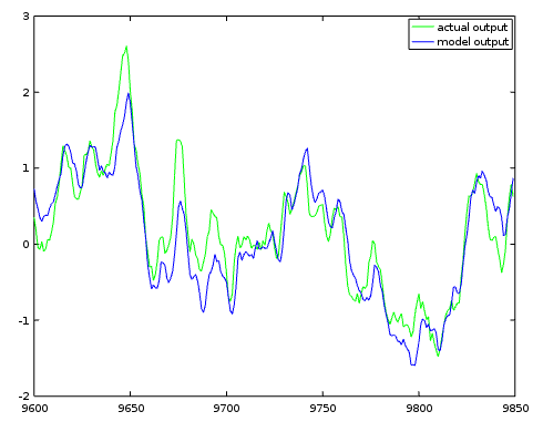
It is judgment day. Compare an arbitrary block of model predictions to the corresponding actual output values.

  Nplot=250;
  Npstart=9600;
  Npend=Npstart+Nplot-1;
  plot(Npstart:Npend,outmat(Npstart:Npend,2),'g', ...
       Npstart:Npend,outmat(Npstart:Npend,1),'b')
  legend('actual system','model system')

The simulation generally tracks the actual system. When the actual system is driven upwards the model tends to be driven upwards as well. When the two trajectories diverge from each other, they eventually tend to drift back together. However, the tracking obtained during the simulation is nowhere close to the match obtained during Least Squares parameter fitting. Keep in mind that the actual system has internal random activity that the model has no way to know about.

 

Can we do better than this?

The quick answer is: probably a lot better, but it will never be perfect.

The only reason we got this far was that we were lucky. This problem wasn't very hard. If it had been harder, and if the model fitting had flopped badly, would anybody read further?

For the best chance of success, there are a lot of important side considerations, and here are some of the coming topics to watch for.

• Efficient representation. Did we make a bad, or possibly horrible, guess about the system order? How can we know?

• Compactness. Is there anything we can do to reduce the massive amounts of data that the least squares fitting problems must manage?

• Data scaling. What impact does the data magnitude have on the quality of the model?

• Sampling. What sampling rates should be used to best observe the system behavior?

• Measurement. What can you do to obtain the best possible measured data for characterizing the system?

• Input noise. How can you best deal with system inputs that are as noisy as the outputs?

• Supplemental signals. How can you take advantage of additional signals besides the ones you specifically need to model?

• Time scaling. How can you represent things that happen fast, or that happen slowly?

• Incremental improvement. Is there any chance of improving the current model to obtain a better one?

 

---