Randomized Test Signals

The idea for quantifying your system's input/output dynamic response is simple. Provide it an arbitrary input signal, in which any sort of input sequence is possible and equally likely. Then, observe how the system responds. Record the sets of input/output data. Do this for a long time, for detecting consistent patterns.

What kind of test signal is appropriate? Here, we will consider a randomized test signal. A randomized signal having desirable properties can be calculated using your favorite mathematical tool. Here, we will use Octave. Then, to drive the real system, the data are sent at regular updating intervals to a digital-to-analog (D-to-A) converter device that will drive your system input.

Start by preparing the randomized data.

 

White noise test signals

An obvious way to calculate a completely unpredictable signal sequence is by using the Octave rand(·) function. This can produce a random value from the range 0.0 to 1.0.

   rv = rand;

It can also produce a long sequence of similar random values, uniformly distributed through the range 0.0 to 1.0, and put them into a vector. For example, to produce a vector with 80000 random terms:

   rv = rand(80000,1);

The D-to-A converter device will expect discrete fixed-point numbers; the range for a typical 16-bit converter is 0 to 65535. However, in most cases, converter devices are configured to operate between balanced "plus and minus" power supplies so that the mid-range value represents output voltage 0. Inputs and outputs can then be expressed as signed integers in the -32768 to +32767 range. (Why isn't it balanced, say between -32768 and +32768? Well, count the number of output codes the device's bits would need to produce for that to be possible.)

The rand function will only give values strictly between 0.0 and 1.0. To span the converter's full digital range 0 to 65535 in a balanced manner, you can scale the values as follows.

   rv = 65535 * rand(80000,1); 

This is a step in the right direction, but the converter hardware requires integer values. The round function will guarantee that the output values are representable as integers.

   rv = round( 65535 * rand(80000,1) ); 

To specify outputs in a balanced "plus and minus" form, reduce each of the original random values by 1/2, leaving the range balanced between -0.5 and +0.5. Then apply scaling and rounding.

   rv = rand(80000,1) - 0.5*ones(80000,1); 
   rv = round(65535 * rv); 

The result after rounding to the nearest integers is a balanced range, spanning from -32767 to +32767.

Producing signals that span the absolute full range of the converters might be a bad idea for the equipment you are testing. To get a more reasonable coverage of the normal operating range, simply scale the magnitudes to a lower range limit. For example:

  % Uniform white noise sequence spanning -24000 to +24000
  testrange = 48000;
  rv = rand(80000,1) - 0.5 * ones(80000,1); 
  rv = round(testrange * rv);

 

Uniform white noise: the dark side of white

The white noise sequence as computed so far has some really good features and some really undesirable ones.

• The randomness of each value means that every value of input is completely uncorrelated every other input value, prior or yet to arise. Any correlation behaviors you see in the system output must be due entirely to the propagation of state information within the system. This is helpful!

• White noise drives your system hard. White noise is a lot like a continuous pounding with impulsive shocks. It can push so hard that the converter devices can't slew fast enough to track the changes, producing a distorted physical signal different than the white noise you thought you were generating. In extreme cases, high level white noise signals could damage equipment.

• Uniform white noise drives every possible signal level equally. In some cases, this "over-represents" the outlier conditions at the fringes of your operating range. As you know, "over-representation" has the same kind of effects as "weighting" the data that go into least squares fitting. You might get a better model for representing normal system conditions by allowing the extremes of the ranges go relatively "under-represented" in favor of more typical operating conditions near the center of the operating range. The white noise property is not violated by using a different distribution of random values beside uniform. One of my favorites variants is the following, producing a triangular distribution^[1] of random values.

  rv = round( testrange * (rand(80000,1) - rand(80000,1)) ); 

 

Reducing noise bandwidth in system testing

The curse of random testing is, well, all of the randomness. The high variance makes it hard to get a consistent result, and huge data sets are needed to distinguish meaningful values from all the variations. If there is something that you can do to reduce the variance, that effort will make it much easier to isolate the consistent system behaviors.

There is a way to do this — use a non-white random test signal.

Here's why you want to do this. Most D-to-A converter devices use a zero-order hold strategy. The digital value is latched; the analog value produced on the output of the converter device sustains until the next digital update is posted. Suppose that you intended to generate a sine wave signal. This is what your actual analog output looks like when posting about 10 updates per waveform cycle (20 percent of the theoretical Nyquist frequency limit for sampled data).

That is chunky but vaguely recognizable as being a "sine wave" shape. All of those "stair-step" transitions rattle your data sets, but at least the point-to-point transitions are smaller than the amplitude of the waveform you are trying to produce. What would this look like with half that many updates per cycle?

This is a really lousy approximation to the original sine wave shape. The chunky transients between sample values are about the same as the magnitude of the sinewave signal you wanted.

The bottom line here is that if you don't have roughly 10 samples per cycle at the highest frequencies you care to represent accurately, the results you will get from D-to-A converters are really lousy. ^[2] There is no point in having input test signals that attempt to force behaviors faster than what your equipment can follow.

Since high frequencies are at best undesirable and at worst harmful in your discrete time models, it is worth keeping them out of your mathematical analysis. And that means it is worth keeping them out of your randomized test signals.

 

Band reduction by digital filtering

A non-white test signal with frequencies roughly uniformly present to about 10% of the Nyquist limit but attenuated beyond 20% of the Nyquist limit can be generated by first constructing an ordinary white noise signal, and then passing it through a digital filter.

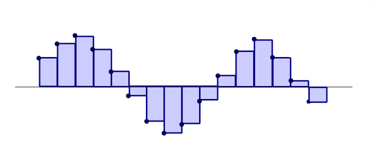
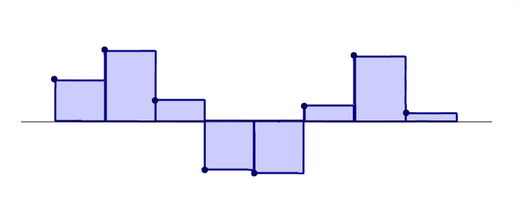
Here is what two randomized signals might look like, the first an unfiltered white noise signal (in green) and the second a filtered signal (in blue).

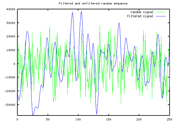
The high-frequency chatter that the system shouldn't track anyway is mostly removed, leaving a much smoother signal.

We'll run a quick FFT spectrum analysis to see how the filtered and unfiltered random signals differ. Take a typical block of white noise random data, and a typical block of the filtered signal as produced by the rsig20 function. (You can generate your own randomized test data by downloading a copy of the rsig20.m function script file.)

    lpsignal = rsig20(2000);  

Calculate the frequency magnitude spectrum for each block, using an fft command, and plot the results for the two spectra using a plot command. This shows the white noise spectrum in green, and the filtered sequence spectrum in blue. Location 200 corresponds to 20% of the Nyquist frequency limit for the sampled data stream.

Beyond 20% of the Nyquist frequency, the signal energy is significantly attenuated. Beyond 30% of the Nyquist frequency there is almost no signal energy present. Roughly 80% of the original white noise signal energy — the part that contributes nothing useful — is suppressed.

The rsig20.m function script file is easy to use, just specify the number of points you want in the sequence block. Be a little cautious about the scaling! Peak values can sometimes extend past the -1.0 to +1.0 range of the original white noise!

 

Side effects

The original random signal values were uncorrelated — white noise. That is, there is no relationship between one test signal value and the next. Is the same desirable property possible with the band-reduced test signal?

Unfortunately, no. Pretty much by definition. If you think about it, knowing that the spectrum contains almost no signal energy at frequencies higher than 20% of the Nyquist frequency limit, you know that some very large and fast transitions that would exist routinely in white noise are extremely unlikely in the filtered signal. Therefore, in the band-limited data there is partial information about what the next signal value is likely to be given the present value. And that means the signal is not white.

However, the test data sequences produced by rsig20 do have one important property: because the filtering is done using a convolution with a vector of finite length, correlation effects will extend only a finite number of points — in this case 20 positions. Any relationship across more sample positions is guaranteed to be an effect of the system response, not an artifact of the test signal.

 

---