Measuring System Correlation

Last time, we discussed how system dynamic response shows up as correlation patterns over time periods spanning a large number of sample intervals. The starting point for such an analysis is obtaining the input/output measurement data — which might sound obvious, but in some ways this is the most challenging part of the process.

Obtaining correlation data

There is a sequence of steps.

Prepare the system

Use the rsig20 function (presented and analyzed in the previous two installments) to generate a random signal sequence. At first, scale the sequence relatively small so that damage is unlikely to your equipment. You can scale up later after you know how large of a test signal is safe. Put a few zero values at the beginning and end of the data sequence so that the digital to analog converter starts and stops at safe levels. Send the sample sequence to your converter/driver equipment and verify that the output levels are suitable.

Collect the data

Pick an appropriate run length N, typically 50000 to a million sample points, depending on the limits of available time. Use the rsig20 function to generate a very long randomized test signal of the selected length. If you are updating the outputs at 1/100 second time intervals, you can process 360000 samples per hour.

Feed the calculated input sequence to your digital to analog converters, which apply the generated signal to your system input terminals. Simultaneously measure the signal as applied at the input terminal of your system and the response as observed at the output terminals of your system. Store the observations as data pairs, input and output, in a large data file. It would be very good to make some short test runs to be completely sure that your setup is working correctly before trying the full-length test.

Exploratory calculations

Before processing all of the data, which is a massive amount of work, experiment on a small subset. This should provide some insights about what to look for in the full analysis.

Run the Octave program. Load the input data and output data into a data matrix dmat. Octave will place corresponding values (input and output channels) into matrix columns; rows represent the progression of these values over time.

Select some number of shift positions Kx for a preliminary correlation study, for example Kx = 2000. Correlation calculations are performed as follows.

    acorr(ishift) = (unshf' * shf) * (1/Kx); 

Repeat these calculations for time shifts of 2 time steps, 3 time steps, and so forth. Plot the results of the preliminary correlation analysis.

    plot (1:Kx, acorr, 'k') 

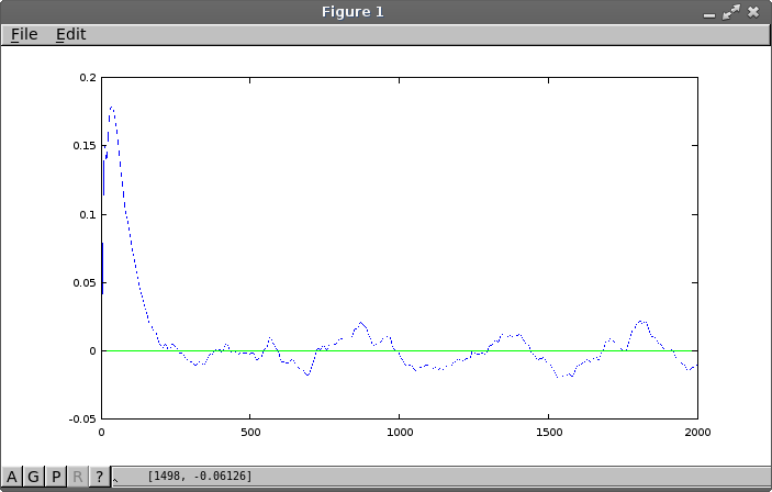
Correlation artifacts are expected over intervals of less than 20 terms, as a side effect of the randomized signal smoothing, so do not expect to find anything relevant there. Beyond that, however, distinct non-random patterns in the correlation sequence are present as expected. These can extend into hundreds of terms.

As the time separation grows larger, correlations should shrink toward the random noise floor. How many terms does it take to get there? Was the number of shift positions Kx selected for the preliminary study a good guess, or should it be a longer or shorter interval? You might want to repeat the preliminary correlation analysis with different Kx values to verify your inference.

In the example plot, there are some clear response patterns and some less clear ones. The dominant correlation peak extends about 250 shift positions. It looks like there is an oscillatory behavior, with a period of 450 samples or so, and we want at least a couple of cycles of this retained in a full analysis. On this basis, an interval of 1200 positions is selected for more detailed study.

The main analysis

The full analysis is very much like the preliminary analysis, with a few adjustments.

• The analysis uses the full data set from the test data file.
• The analysis uses the number of shift positions K selected during the preliminary analysis. For our example, K = 1200 is selected.
• The number of product pairs the data set will support is N - K, to avoid shifting beyond the end of the data set.
• An autocorrelation analysis selects data from the output data column for both the shifted and unshifted sequences.
• A crosscorrelation analysis selects shifted output data and unshifted input data for the data sequences.
• For both cases, note that the shifted data is always taken from the output data.
• Calculate and store the correlation values over the selected range of time shifts.

Here is an example plot, showing a cross-correlation from a one hour run of 360000 samples. That is, it shows the degree of linear relationship between the output data and input data for each time period.

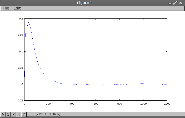
Some features to notice:

• A dominant exponential decay of duration about 350 sample intervals
• An extended oscillatory pattern with cycle around 220 sample intervals, at a lower level than what seemed present in the exploratory study
• An initial exponential rise of duration approximately 100 samples
• An unusual and possibly spurious fast oscillation of duration around 30 samples

Correlation and state behaviors

Yes, but what does all of this mean?

From this point on, the analysis becomes more qualitative and a little less obvious. Fortunately, we don't need to precisely nail down what the system is doing; the immediate goal is just to estimate how many things the system is doing to get an appropriate number of state variables for a model. But what things? We will start there next time.