State Observers: Design

Last time we discussed how to design observer equations, but since the whole concept was probably theoretical and unfamiliar, we need to do some good old fashioned number hacking to design a set of observer equations and give them a workout.

The observer equations

We will start from where we left off, with a reasonable model that was clearly under-performing because of noise. We developed some design equations, and determined that we needed to select a matrix F by some process to satisfy the following condition.

Basically, that just says that the magnitudes of all the matrix eigenvalues are less than 1.0. The matrix (A - F C) then becomes the state transition matrix E for the observer equations:

where the values of state estimates z are supposed to track the internal states of the system as well as possible.

Setting up

As noted last time, if the model is stable initially, the observer equations can start with an observer gain F of 0. But you can see that in this situation no output information is used, and the state observer produces nothing useful. Here is a state equation system that we have seen previously.

Amat =
   0.98900   0.00000   0.00000   0.00000   0.00000   0.00000
   0.00000   0.93000   0.00000   0.00000   0.00000   0.00000
   0.00000   0.00000   0.98960  -0.01477   0.00000   0.00000
   0.00000   0.00000   0.01477   0.98960   0.00000   0.00000
   0.00000   0.00000   0.00000   0.00000   0.92395  -0.29938
   0.00000   0.00000   0.00000   0.00000   0.29541   0.92115

Bmat =
   1
   1
   1
   0
   1
   0

Cmat =
   0.1232020  -0.1491940   0.0473420   0.0278580  -0.0145235   0.0036879

Initialize an empty observer system gain matrix.

Fmat = [ 0.00; 0.00; 0.00; 0.00; 0.00; 0.00 ];

Optional, calculate the stability boundary for plots. To be stable, the magnitudes of the eigenvalues of the observer equation matrix must all have magnitudes less than 1.0. I find it useful to compare their locations to this stability boundary.

% Calculate stability boundary points for plotting
for iterm=1:61
  sinval(iterm)=sin(pi*(iterm-31)/(3*60));
  cosval(iterm)=cos(pi*(iterm-31)/(3*60));
end

The search for the gain matrix

Set up an Octave script that defines the following operations.

% Calculate proposed observation matrix 
Emat = Amat - Fmat * Cmat;

% Calculate its eigenvalues
evec = eig(Emat)

% Display the eigenvalues and their magnitudes
magnitudes = abs(evec)'
evr = real(evec);
evi = imag(evec);

% Display the eigenvalues on a plot to evaluate stability
plot(evr(1:6),evi(1:6),'k*', cosval,sinval,'r')

Now you can run this script each time you want to try a new proposed observation gain.

In this case, there is a single output value produced by the state equations with corresponding actual output values available in the input/output dataset. This makes things a little easier and a little harder. It is easier because the "gain matrix" becomes a "gain vector" and there are fewer terms to adjust. It is harder because a single output variable produces more constrained behaviors and there is not as much that you can control in your results.

Running the script without any Fmat adjustments, the following shows the initial eigenvalue set.

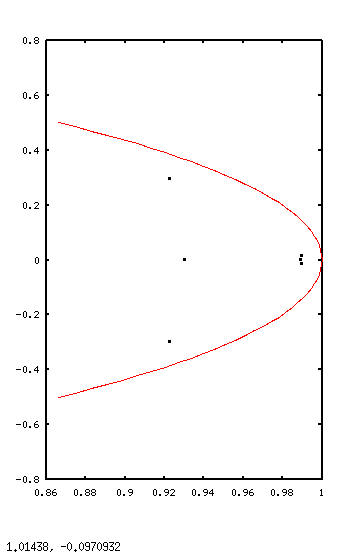
The biggest problem is the cluster of eigenvalues with magnitude about 0.99. That indicates very a very slow convergence rate for the state estimates. There is also one eigenvalue with magnitude about 0.92 which is maybe a shade too small, which could allow a little too much noise to disrupt the short-term convergence of the state estimates. If achievable, eigenvalues with magnitudes in the range 0.94 to 0.97 or so would be the most desirable compromise between speed of convergence and noise sensitivity.

The red curve is the stability limit for sampled systems. If any of the eigenvalues pass beyond this curve, errors will not settle and the state tracking errors will grow without bound.

I tried adjusting the terms of the Fmat matrix one at a time, looking for a rough idea of the sign and a reasonable magnitude for each term. Here are my notes from these experiments, accumulated in the form of Octave comment lines.

%Fmat = [ 0.2; 0; 0; 0;  0;   0 ];  % Shifts middle eigenvalue pair
%Fmat = [ 0; 0.2; 0; 0;  0;   0 ];  % Shifts lower real eigenvalue
%Fmat = [ 0; 0; 1.3; 0;  0;   0 ];  % Spreads eigenvalue cluster
%Fmat = [ 0; 0;  0; -.5; 0;   0 ];  % Shifts high eigenvalue pair
%Fmat = [ 0; 0;  0;  0; -0.5; 0 ];  % Shifts low eigenvalue pair
%Fmat = [ 0; 0;  0;  0;  0; -10 ];  % Shifts low eigenvalue pair

The indicated numbers seemed reasonable when applied individually, but applying all at the same time is probably too much. So I scaled the values all back by a factor of about 0.5, and then combined the terms into a single Fmat matrix. This showed a clear improvement.

From there, I continued adjusting terms of the Fmat one or two at a time, and recalculated the observer matrix eigenvalues. Here is the combination that I liked the best.

 
Fmat = [ 0.25; 0.1; 1.0; -0.9; -1.0; -4.0];  

evec =
   0.92763 + 0.26319i
   0.92763 - 0.26319i
   0.94819 + 0.03991i
   0.94819 - 0.03991i
   0.97687 + 0.00278i
   0.97687 - 0.00278i

ans =
   0.96425   0.96425   0.94903   0.94903   0.97687   0.97687

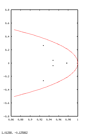
This was about as good as I could get it, and in a typically acceptable range. Let's try it.

Applying the state observer

Obtain a sequence of input and output data. For purposes of this test, the state transition equations are used to simulate the actual system by injecting some random noise into each of the state variables after each update.

  % Noise affects actual system state and output
  realout = Cmat * Xnoisy;
  Xnoisy = Amat*Xnoisy + Bmat*indat(iterm) + noise(iterm);

Now apply the state equation model in the usual manner for a simulation. This calculation is given exactly the same input data, but not the hidden internal system noise.

  % Simulate the normal application of the state transition model
  simout = Cmat * Xstate;
  Xstate = Amat*Xstate + Bmat*indat(iterm);

In parallel with the state transition equations, also update the state observer equations in an attempt to estimate the system's internal states from actual output values observed.

  % Use input and output data to update observer equations
  Zstate = Emat*Zstate + Fmat*realout + Bmat*(indat(iterm));

Now we have a problem. We have two different estimated values for what the next state will be. If we trust the original state transition equations, the next state of the system is Xstate. But if we trust the state observer equations, the state of the system is Zstate. How can we resolve this inconsistency?

I have chosen to trust the observer estimate about twice as much as the state transition estimate. You can try adjusting this ratio as you wish.

  Xstate =  0.35*Xstate + 0.65*stateZ ;

Now, instead of the original Xstate vector, I will substitute this hybrid value that includes the corrections.

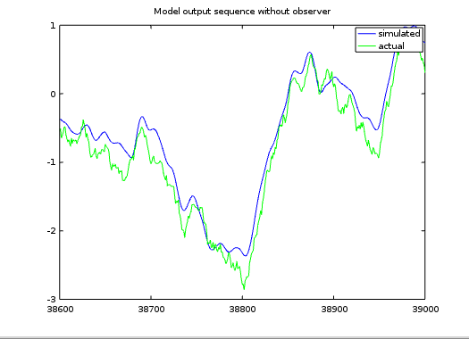
For comparison, here is the sequence of output values from the noise-disturbed system without any observer corrections applied.

Now, here is the modified result after introducing state corrections based on the state observer estimates.

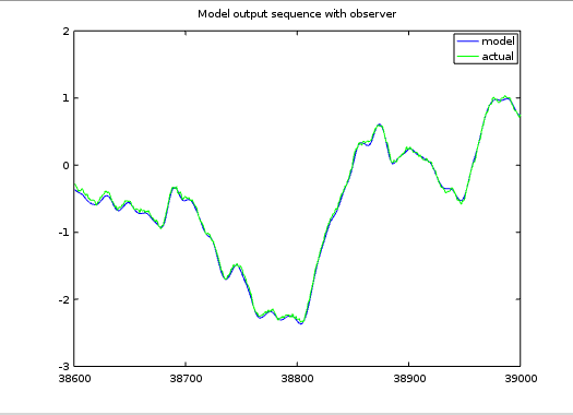
Is it starting to become apparent how the state observer can be beneficial?

Coming events

There is a very strong relationship between the observer equations and the state transition equations. That should be expected, since the state transition matrix contributes a significant part of the information that goes into the observer matrix design. Since linear effects are additive, perhaps we can reorganize the observer equations to distinguish the parts of its behavior that are the same as the state transition matrix, and the parts of its behavior that are different. Now you're starting to think like Kalman...

But before we go too far in that direction, there are other considerations we need to think about with regard to observers. We will pick that up next time.