Minimalist Observer: the Alpha Beta Filter
Developing Models for Kalman Filters
Previously, we considered what could happen if the observer strategy was applied using a state transition model of reduced order and low parameter accuracy. We found that the output tracking could still perform remarkably well (under the circumstances). Last time we discussed a more efficient two-step implementation. This time, we will push the goal of simplification to extremes — and find that there is possible benefit even then.
The presumptive model
The system is presumed to exhibit a high degree of momentum. That is, unless something happens to change things, the system will continue doing what it did in the past, unchanged.
- The output of the system is presumed at each step to be the same as it was on the previous time step.
- If the output is changing, the rate of change is presumed to be the same as it was at the previous time step.
These two assumptions are inconsistent — the system
output can't be holding a steady position while at the same time
changing position at a steady rate. We can reconcile the conflict
by noting that for a system with constant change rate v,
and with a sampling time interval ΔT, the
constant rate will produce a predictable consistent change in position
during each time step. ("The position change is the integral of the
constant velocity over a small time step, v ΔT.")
Define the state vector as
where
    p    is the "position" of the system output
    v    is the "velocity" of the system output change
Presume no knowledge of the system's input. With zero known inputs, we can dispense with the usual input coupling matrix terms. Lacking input information, the model prediction will be that, once started into motion, the system will proceed at a steady rate forever.
To further simplify, assume that the "position" and "velocity"
state variables are normalized. Since the system is linear, this
means that a final scaling factor c, taking the place
of the usual output observation matrix, will be helpful for the
output calculations to "undo" the normalization. Otherwise, use
the normalized position variable. Consequently,
separate calculations for "output observation" can be omitted.
These relationships provide the forward projection step, producing the intermediate next state estimates.
Applying the observer
Working alone, with no input at all, this dynamic model will not
predict anything directly useful. So now design an observer for it.
The observer will apply
corrections that are proportional to the tracking error for the state
variable. The two multipliers are called α and
β. The observer corrections are then applied using
a two-step update as follows, to obtain the adjusted state estimates
for the next step.
Applying the two-step projection and correction process one term at a time to a sequence of noisy data can yield an output sequence that is less noisy, so this process can be called a filter. It takes its name alpha beta filter [1] from the two observer gain coefficients.
There is no general theory to guide you for the selection of the two observer gain values. But heck, the observer design process as seen so far has been a cut-and-try exploration anyway. This isn't that much worse.
The strategy is pretty easy. Pick a small value for the
α parameter. Stream some data through the
alpha-beta filter. Do you like the tracking results you see? Then
maybe adjust the value a little more. Then try the β
term, making similar adjustments. Repeat, try and test again, trading
off changes in one variable for changes in the other, until you
get the best results you can find (where best is defined as
what looks good to you).
An experiment
I grabbed one of the simulated noisy systems from a previous installment. It doesn't matter what it is, because the alpha beta filter doesn't know anything about where the data comes from. Here is the filter state matrix that I used for this experiment.
ABmat = [ 1, 0.04; 0.0, 1.0 ];
These were the alpha beta filter gains that I decided upon.
alpha = 0.20;
beta = 0.30;
ABgain = [ alpha; beta ];
And these were the filter calculations I used in the processing loop.
   % Update the alpha beta filter
   pv = ABmat * pv;
   yerr = yout-pv(1);
   pv = yerr * ABgain + pv;
   about = pv(1);
The results? Here is a plot of the output trajectory as produced by the alpha-beta filtering, superimposed on the original noisy data set.
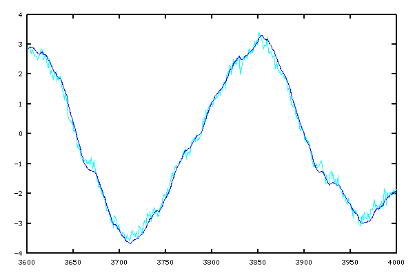
This is hardly perfect. Having no information about the system inputs, it has trouble tracking quick transitions accurately. Having little useful state information, it isn't effective at correcting a tracking error until the error is already well established, causing a tendency to lend to lag the actual system trajectory by a small amount. However, the amount of improvement is remarkable given the general lack of rigor and effort.
This could be very useful, but you will need to be the judge of when. Typical applications are for data smoothing when it is helpful for removing lots of short-duration noise without too much effort, or cleaning up noisy measurements of slowly-changing variables, such as thermal drift.
Extensions
Here are a couple of variations that you can consider.
- The alpha beta filter suffers from not having any input information. That information is often readily available. If so, you might as well use it to your advantage. Apply an input coupling multiplier parameter to the input values, and add the new term into the second alpha beta filter state, as a sort of crude "accelerator" approximation. Then tune the input coupling coefficient along with the alpha and beta parameters for best results.
- For some systems, the behavior is better approximated by constant acceleration than by constant velocity. A third state can be added, with the second state obtained from the new third state by integration, in a manner similar to the way the first state is obtained from the second state. Then the observer will need three adjustable parameters, leading to the alpha beta gamma filter.
Better theoretical basis?
There is something a little unsatisfying about the cut-and-try process used to design observers. There should be something a little more systematic, if not producing a perfect design, at least getting close quickly.
An observer has a choice.
- It should use high observer gains to correct tracking errors quickly when model predictions are accurate and noise levels are low. (These higher gains will force lower eigenvalues in the observer matrix.)
- It should use lower observer gains, trusting prior observer estimates of the state more and the corrections less, when the measurements of the system output exhibit higher noise levels so that no individual observation can be fully trusted.
Somewhere between these two strategic extremes, there should be a place that is a best balance between speedy state corrections and noise sensitivity. Is there a way to systematically find that balance? To address this question, we will need to more carefully consider how to characterize the system noise, and that topic launches our new direction for next time.
[1] See the Wikipedia article https://en.wikipedia.org/wiki/Alpha_beta_filter for a relatively complete presentation of this subject. Though starting out reasonably (I consider it some of my better work), supplemental material about "optimal" gain choices seems rather silly. Take a barely plausible heuristic model, apply questionable statistical assumptions, and then mathematically optimize it? What exactly does that accomplish? Seriously, if you have enough understanding to obtain a reasonable noise model, you will probably do better with a proper Kalman Filter.