Overview
Other sites:
This learn by doing tutorial shows how symbolic computations with Maxima can be used to facilitate circuit analysis for electronic networks. It is assumed that you have Maxima installed and running. (If not, what's the matter with you?) It is also assumed that you know how to formulate the equations for the electronic circuit you wish to analyze. If you don't, that might not be an insurmountable difficulty after the brief introduction to follow, but plan on a little extra homework.
Why consider Maxima when there are computational tools such as SciLab, MatLab, Octave or Spice that can calculate various circuit transfer and driving-point characteristics? For applying numerical methods to solve sets of simultaneous network equations and obtain numerical results, given component values, these work great. But suppose you don't know the component values — and determining how to choose these is the whole point of the study. The symbolic solution approach can give you a closed-form expression presenting the desired network characteristic as a direct function of the component values. (And once you have this formula, you have gained a tremendous advantage for further studies with your numerical calculation tools.)
Getting the network equations
As stated previously, this presentation is not intended as a tutorial on network analysis. However, to provide some background information on the process used to build the network equations...
The electronic network equations are typically obtained by repeated application of the following principles.
- Kirchoff's Current Law - The sum of all currents flowing into a circuit node must equal the sum of all currents flowing out. (Otherwise, that node would accumulate charge and the voltage would spin off to infinity.)
- Kirchoff's Voltage Law - The sum of the voltage differences across components around any closed loop must be zero. (Otherwise, just by following around the loop, you would find that one place has two different potential energies simultaneously, an absurdity.)
- Component Constraints - The current through each element is the difference in voltage across the element divided by the impedance of the element. (For resistors, the impedance is considered constant at all frequencies, and is called resistance. The impedance varies in proportion to frequency for inductor components, and inversely to frequency for capacitor components.)
In general, as you collect network constraint equations, as long as each added constraint equation involves some network element that was not covered in any previous constraint, and this is continued until every element is covered, you will obtain an equation set that is linearly independent. Then, apply the component constraints so that every current passing through a component determines the voltage difference across it — or the reverse.
The network equations are often extended to include active elements. The normal "asymptotic" assumption for these is that the amplifiers are able to sustain their gains through the bandwidth of signals that you care about. (Advanced problem: how can you add additional network constraints to study what happens outside of this range?) Under the normal assumptions, internal or external amplifier feedback will guarantee the following conditions to very close approximation:
- For a high gain operational (voltage) amplifier, feedback will force the voltage at the inverting input of the amplifier to equal the voltage at the non-inverting input of the amplifier. The amplifier inputs draw insignificant input current. The output voltage of the amplifier will be whatever is required to force the input conditions.
- For a transconductance (current) amplifier, the feedback will force the current flowing into the inverting input of the amplifier to equal the current into the non-inverting input of the amplifier. The output voltage of the amplifier will be whatever is required to produce this condition.
- For a unity gain buffer amplifier, the output voltage of the amplifier is forced to match the input voltage of the amplifier. There is insignificant current draw into the amplifier. The amplifier output drives whatever current is required to produce the voltage tracking condition.
- ... and so forth for other styles of high-gain active devices.
Maxima features required
One of the joys and nightmares of using Maxima is the sheer number of commands available (and that is only the standard set). Fortunately, for purposes of circuit analysis, you only need a very small subset of these. Here is a quick survey, but don't worry about memorizing all of these details immediately, you will see them again very shortly.
( ) |
Parentheses, group expression terms, typically so that various operators can be applied to the combined result of a sub-expression. |
list[ indx ] |
Indexing notation, to extract one of the sub-expressions of
an array |
: |
Colon operator, assign an expression to a symbol, for later reference. The primary application will be to enter a network constraint equation or complicated sub-expression. If Maxima has a prior definition for one of the right-side terms, it will automatically apply that definition as it processes the expression. |
' |
Single apostrophe prefix, tells Maxima to defer substitutions even if the expression contains symbols that Maxima already knows about. If you omit this, Maxima might substitute for terms prematurely, or in a counterproductive manner. |
'' |
Two apostrophe prefix, tells Maxima to evaluate the expression and make all of the symbolic substitutions it knows about — somewhat the opposite of the single apostrophe prefix. You can use this to apply an accumulated set of symbol definitions to an expression all at once. |
% |
A shorthand for the result produced by Maxima's last operation. |
rhs(expr) |
Given a constraint expression |
solve(expr,term) |
Solve function. For an equality constraint expression |
subst(new,term,expr) |
Symbolic substitution. Insert the expression |
ev(expr,sub1,...,subN) |
Apply a list of substitution expressions |
ratsimp(expr) |
Attempt to simplify an expression to reduce it to a ratio of two sub-expressions. Very useful for linear network analysis, since many network characteristics for linear networks turn out to be rational. |
The network example
The network configuration to analyze is shown in the following figure.
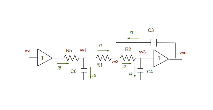
This is a variant of a classic Sallen-Key lowpass filter. A typical
Sallen-Key stage has a first- or second-order characteristic; the goal here is to
determine the transfer voltage gain characteristic vvo / vvi
after adding additional components to extend the network to a third
order filter.
For identifying network elements, node voltages (input, three internal junction points, output) are assigned names, shown in red in the illustration. Currents through network branches are assigned the names shown in green, with an associated green arrow showing the reference direction of the flow. The electronic component values (resistors R5, R1, R2, and the capacitors C6, C4, and C3) are not known. The goal is to determine how to select these component values to achieve a known, desired transfer characteristic.
Some observations about this network:
- The unity gain amplifier on the front end guarantees that there are
no stray currents flowing back into the driving source
vvifrom the filter network. - The unity gain amplifier on the output guarantees that any current
required to drive the next stage at output voltage
vvodoes not interfere with current flows in the filter network components. - The unity gain of the output amplifier guarantees that voltage
vvotracks the voltagevv3. - The rest of the network is constrained by the three current junction
nodes between the input buffer amplifier and the output buffer amplifier,
associated with voltages
vv1,vv2, andvv3.Thus, we can use the node current balance equations to build the network equations. (Though there are lots of other ways to do it!)
Putting Maxima to Work
The displays I show in this section are the commands in the original form as I entered them (not Maxima's formatted echo of those commands!), followed by the displays of results that Maxima produces.
Start up Maxima. To prevent any confusion with past evaluations, clear everything.
                    kill(all);
(%o0)                                done
Next, begin entering the network constraint equations. (Follow these in the network diagram.) In this case, node-current constraints are used. Each constraint is assigned a name. To prevent any early and unexpected substitutions of variables, the "tick notation" (hyphen) is used to temporarily suppress symbolic substitutions. You can see that Maxima collects the expressions without altering anything.
                    node1 : '(i5 = i6 + i1)
(%o1)                            i5 = i6 + i1

                    node2 : '(i3 + i1 = i2)
(%o2)                            i3 + i1 = i2

                    node3 : '(i2 = i4)
(%o3)                            i2 = i4
Similarly enter the unity-gain output amplifier constraint.
                    node4 : '(vvo = vv3)
(%o4)                            vvo = vv3
Now enter the component constraints, to relate the currents appearing in the node constraint equations to the voltages across elements. The "tick" operators are omitted. We don't need to worry about suppressing symbolic substitutions here, because the expressions contain only new symbolic terms.
                    i5: (vvi - vv1)/z5;
                                   vvi - vv1
(%o5)                              ---------
                                      z5
                    i6: (vv1) / z6;
                                      vv1
(%o6)                                 ---
                                      z6

                    i1: (vv1 - vv2)/z1;

                                   vv1 - vv2
(%o7)                              ---------
                                      z1

                    i3: (vvo - vv2)/z3;
                                   vvo - vv2
(%o8)                              ---------
                                      z3

                    i4: (vv3)/z4;
                                       vv3
(%o9)                                - ---
                                       z4

                    i2: (vv2 - vv3)/z2;
                                   vv3 - vv2
(%o10)                             ---------
                                      z2
Having now verified that all of the network equations are loaded and correct, we can get down to the business of solving.
The first thing we can notice is that the node4 constraint makes
the output voltage vvo and the node3 voltage vv3
redundant. We can substitute symbol vvo everywhere that the
vv3 symbol is seen.
                    i4 : subst(vvo, rhs(node4), i4)
                                       vvo
(%o11)                                 ---
                                       z4

                    i2 : subst(vvo, rhs(node4), i2)
                                   vv2 - vv0
(%o12)                             ---------
                                      z2
Voltage vv3 no longer appears in any of the other three network
equations, so we can disregard the node4 constraint from this point onward.
Now, we can turn Maxima loose to apply all of the component constraints into all of the terms in the other node equations.
                    node1: ''node1;
                          vvi - vv1   vv1   vv1 - vv2
(%o13)                    --------- = --- + ---------
                             z5       z6       z1

                    node2: ''node2;
                       vvo - vv2   vv1 - vv2   vvo - vv2
(%o14)                 --------- + --------- = ---------
                          z3          z1          z2

                    node3: ''node3;
                               vv2 - vv0     vvo
(%o15)                         --------- = - ---
                                  z2         z4
We see that node1 now relates the voltages vvi,
vv1 and vv2. If we solve this constraint
to obtain a value for vv1, this expression can be
substituted for the vv1 terms in all the other node
equations. First, we need to get that solution. The result comes
back as the first element in the solution array, so there
is an extra step to extract it.
                    solve(node1, vv1)
                    node1: %[1];
                                (vv2 z5 + vvi z1) z6
(%o16)                   [vv1 = --------------------]
                                (z5 + z1) z6 + z1 z5

                                (vv2 z5 + vvi z1) z6
(%o17)                    vv1 = --------------------
                                (z5 + z1) z6 + z1 z5
Shifting attention now to node2, we see that it relates the node
voltage vv2 to the voltages vv1 and vvo.
We already have an expression for vv1 in terms of vv2
and vvo. Using the subst function, replace each
instance of vv1 in node2.
                    node2 : subst(rhs(node1), vv1, node2);
              (vv2 z5 + vvi z1) z6
              -------------------- - vv2
              (z5 + z1) z6 + z1 z5         vvo - vv2   vv2 - vv0
(%o18)        -------------------------- + --------- = ---------
                          z1                  z3          z2
Comparing this to the previous node2 equation in output line o14,
we can see that the vv1 term has been replaced. The term
vv1 no longer appears in either the node2 or node3 equations,
so we can disregard the node1 constraint from now on.
The same strategy can be employed again at node2, this time solving to obtain
an expression for the vv2 voltage.
                    solve(node2, vv2);
                    node2: %[1];
(%o19) [vv2 = (((vvo z3 + vvo z2) z5 + (vvi z2 + vvo z1) z3 + vvo z1 z2) z6
 + (vvo z1 z3 + vvo z1 z2) z5)/(((z3 + z2) z5 + (z2 + z1) z3 + z1 z2) z6
 + ((z2 + z1) z3 + z1 z2) z5)]

(%o20) vv2 = (((vvo z3 + vvo z2) z5 + (vvi z2 + vvo z1) z3 + vvo z1 z2) z6
 + (vvo z1 z3 + vvo z1 z2) z5)/(((z3 + z2) z5 + (z2 + z1) z3 + z1 z2) z6
 + ((z2 + z1) z3 + z1 z2) z5)
Substitute this into the node3 constraint, replacing the vv2
terms in that expression.
                    node3 : subst(rhs(node2), vv2, node3);
(%o21) ((((vvo z3 + vvo z2) z5 + (vvi z2 + vvo z1) z3 + vvo z1 z2) z6
 + (vvo z1 z3 + vvo z1 z2) z5)/(((z3 + z2) z5 + (z2 + z1) z3 + z1 z2) z6
                                          vvo
 + ((z2 + z1) z3 + z1 z2) z5) - vvo)/z2 = ---
                                          z4
This is messy, but it involves only the component impedances and
the two voltage variables that we care about, vvi and
vvo. Solve the node3 expression to obtain an expression
for vvo. The filter transfer function ratio we want
is then equal to vvo / vvi.
                    solve(node3, vvo);
                    tr: %[1] / vvi;

(%o22) [vvo = (vvi z3 z4 z6)/(((z3 + z2) z5 + z3 z4 + (z2 + z1) z3 + z1 z2) z6
                                          + (z3 z4 + (z2 + z1) z3 + z1 z2) z5)]

       vvo
(%o23) --- = (z3 z4 z6)/(((z3 + z2) z5 + z3 z4 + (z2 + z1) z3 + z1 z2) z6
       vvi
                                           + (z3 z4 + (z2 + z1) z3 + z1 z2) z5)
To make this expression more useful, make two adjustments. First,
express impedances for resistors as being simply a constant resistance
value; and express impedances for capacitors as being inversely
proportional to complex frequency s. There are no inductor
elements. We can apply these substitutions for all of the impedance terms
simultaneously using an ev operation.
      tf: ev(%, z1:r1, z2:r2, z3:1/(c3*s), z4:1/(c4*s), z5:r5, z6:1/(c6*s));

       vvo                    r2 + r1      1
(%o24) --- = 1/(c3 c4 c6 (r5 (------- + -------- + r1 r2)
       vvi                     c3 s            2
                                        c3 c4 s
                                  1           r2 + r1      1
                             r5 (---- + r2) + ------- + -------- + r1 r2
                                 c3 s          c3 s            2
                                                        c3 c4 s            3
                           + -------------------------------------------) s )
                                                c6 s
Looking at this, I apologize for calling any of the earlier expressions
messy. But we don't have to leave things this way. We can use the ratsimp
function to request an algebraic simplification that turns out to give exactly
the kind of expression we want.
                    tf : ratsimp(%):
       vvo                         3
(%o25) --- = 1/(c3 c4 c6 r1 r2 r5 s  + (((c4 c6 + c3 c4) r2 + c4 c6 r1) r5
       vvi
                                      2
                      + c3 c4 r1 r2) s  + ((c6 + c4) r5 + c4 r2 + c4 r1) s + 1)
This shows exactly how each term in the network transfer function depends
on component values at each complex frequency s. Determine how
you would like your filter to respond — for example, use the mathematical
characteristic for a third-order Butterworth filter to determine what the values
of the transfer function coefficients must be to produce a "maximally flat"
characteristic at frequency zero and a rolloff at a desired high frequency band
edge. Then, select component values to accomplish this.
To experiment further with this particular filter, download
the Maxima script file
and change the name to SalKey3.mac. You can then use the
Maxima batch command to run the file directly.
Conclusion
This "interactive" example demonstrates the basic ideas of how to solve electronic network analysis problems symbolically with Maxima:
- Enter network topology constraint equations, avoiding premature symbolic substitutions.
- Enter component constraint equations, again avoiding premature symbolic substitutions.
- Apply active element constraints and eliminate redundant, dependent variables.
- From a network constraint equation, solve for one of the internal variables. Substitute for this internal variable to eliminate it from all of the other network constraint equations.
- Repeat in a similar fashion until left with a constraint expression having only component values and the desired input and output variables remaining.
- Calculate the output-to-input ratio to obtain the network characteristic you were seeking.
- Apply algebraic simplification to put the result into a usable form.
- Use this result to advantage for other numerical studies of your network.
Unfortunately, Maxima has no way of knowing which variables in your network equations are the important input and output quantities you are studying. Maxima also has no way of knowing "what should be substituted for what" to reduce your network equations to the form you want. So you must provide that guidance, telling Maxima which variables to substitute, for what, and where. Fortunately, that is the interesting part; the tedious algebraic manipulations are all done for you by Maxima.