Introduction
Other sites:
This note discusses methods for estimating the values of the derivatives of an unknown function, given measured equally-spaced function values with a certain amount of random measurement noise. I was interested in a curvature analysis for which a second derivative would be useful. I knew that this would be a challenging problem, but I was surprised to find that the numerical methods usually suggested for this are really not very good.
Conventional approaches and extensions
As an example of the drawbacks of some of these commonly cited methods, consider the classic central differences[1] "exact fit" polynomials. The idea is that if you construct a polynomial curve that passes through the data points, then the derivative of this polynomial is an estimate of the derivative of the underlying function. The following plot shows what happens if you apply this approximation strategy to estimate the second derivative of a cosine wave with peak amplitude 1, and then you adjust the frequency of the cosine wave. The green curve shows what the correct response magnitude should be at each frequency, while the blue curve shows what the approximation formula calculates.
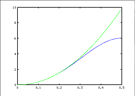
  f''(0) ≅  [ 2.0 f(-3h) - 27.0 f(-2h) + 270.0 f(-h)
             -490.0 f(0) + 270.0 f(h) - 27.0 f(2h) + 2.0 f(3h) ] * 1/(720.0 h2)

    where h is the interval between samples
While at first this seems like a very good approximation, it has a severe problem — its noise sensitivity. A normalized frequency of 1.0 represents the sampling rate of 1 sample per 1 time interval. The Nyquist limit, above which frequencies can no longer be uniquely distinguished, falls at frequency 0.5, so this is the maximum range plotted. A frequency of 0.1 means that an "up and down" variation is spanned by 10 samples in the data sequence. This sort of variation is probably meaningful and should be analyzed to high accuracy. A frequency of 0.2 means that the "up and down" variation is spanned by 5 samples in the data sequence. Patterns covered by 5 or fewer points are more likely to be noise than anything meaningful, so the processing should suppress this noise rather than making it worse.
Previous results
Lanczos proposed a method described by R. W. Hamming[2]:
"... a low noise differentiation filter is proposed that has (a) a unit slope at f=0 and (b) minimizes the sum of squares of the coefficients."
Large gain does tend to follow from filters that have large terms, so a filter that does not have these should be quieter... but the accuracy is poor at the low frequencies where accuracy matters.
Pavel Horoborodko presented another approach[3] that produces derivative estimators that are very good as frequencies close to 0.0 and, for the filter size, remarkably quiet at very high frequencies. However, the accuracy is compromised and there is still a lot of noise passing through in the middle range. The following graph illustrates the frequency response characteristic in blue for one of these second-derivative filter designs.
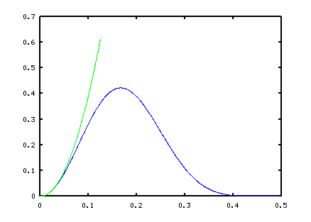
  f''(0) ≅  [ 1.0 f(-4h) + 4.0 f(-3h) + 4.0 f(-2h) - 4.0 f(-h) - 10.0 f(0)
            - 4.0 f(h) +  + 4.0 f(2h) + 4.0 f(3h) + 1.0 f(4h) ] * 1/(64.0 h2)
You can see the excellent noise rejection above frequency 0.4, and excellent accuracy to roughly frequency 0.025 at the low end. However, the accuracy can be seen to be poor at frequencies approaching 0.1, while a lot of noise is amplified in the 0.2 to 0.3 frequency range. If the filter order is increased (thus adding more terms), this gives flatter low-end response, and more high-frequency rejection, but in general the accuracy in gets worse.
A "naive" filter and unexpected result
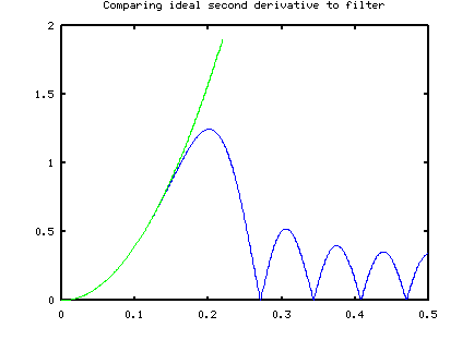
I tried a naive approach to this problem. The classical polynomial-based estimators become sensitive to noise because their approximation curves exactly match every measurement point, noise and all. A "standard" noise suppresion technique is to fit a smooth curve to the data set, without attempting to match the values exactly. What if this alternative idea is used to fit a polynomial to the data for purposes of a derivative approximation? Low order polynomial approximations have limited curvature, hence a natural tendency to not track high frequencies, and this should somewhat limit the response to high-frequency noise. However, there is nothing to explicitly force noise rejection. It just happens naturally — or not! Here is the result of a typical design.
 % To frequency 0.10 of sample rate with 0.01% peak error
     filter2 = [ ...
    -0.0025402   0.0224100  -0.0779679   0.1199416  -0.0274123  -0.1321265 ...
     0.0337787   0.2130250   0.1305009  -0.1379610  -0.2832965  -0.1379610 ...
     0.1305009   0.2130250   0.0337787  -0.1321265  -0.0274123   0.1199416 ...
    -0.0779679   0.0224100  -0.0025402 ] ;
This was rather surprising. Using approximately twice as many terms, this estimator much better accuracy in the desired frequency range, while providing a helpful if not ideal level of noise attenuation at high frequencies. The following plot compares the two methods given a noisy data sequence consisting of a sinusoidal input frequency of about 0.02 contaminated with broadband (white) noise. The ideal response is in green. The "robust low noise" estimate is in red. The "naive least squares" estimate is in blue.
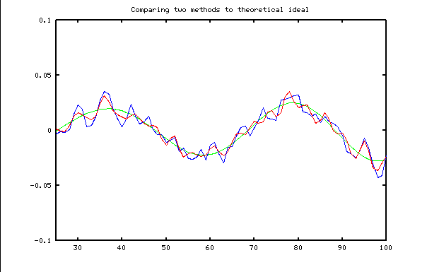
This naive "least squares design" is accurate within 0.01% (relative to an input magnitude of 1.0) through frequency 0.10. The response is potentially useful beyond that, though not as accurate. It is not quite as good as the Holoborodko formulas for frequencies very close to zero.
I was starting to think maybe this was a useful idea — perhaps a relatively minor adjustment could further reduce the high frequency noise response and produce a really superior design. Unfortunately, I couldn't find any reasonable way to do this. This approach was at a dead-end.
Another dead-end street
So I turned my attention to a frequency-based approach. I knew that a derivative operator would show a negative symmetry, which would correpond to a harmonic series of sine waves. If I could find a good sine-series approximation to the ideal frequency response curve, this frequency-oriented approach should produce a good filter design. It is straightforward to include additional "penalty" terms encourage a nearly-zero response at high frequencies.
I won't go through the details of this direct discrete sine wave fitting aproach. It offered some improvement, but not the breakthrough I was looking for.
Two other approaches eventually showed more promise. If you need the best of the best, proceed directly to the FFT Design Method page. While the properties of these estimators are appealing, the manual tweaking necessary in the design process is tedious; and then, the resulting filter takes significantly more computation. For another design approach that produces more economical estimators that are almost as good, see the Optimal Design Method page.
Footnotes:
[1] See for example Finite Differences at Wikipedia.
[2] The classic "Digital Filters" by R. W. Hamming covers the derivative estimator filters from a frequency analysis point of view, and describes the Lanczos low-noise designs in "an exercise."
[3] You can find Pavel's pages at:
http://www.holoborodko.com/pavel/numerical-methods/numerical-derivative/smooth-low-noise-differentiators/