A Screening Test for Latin Square Randomness using Matchings
Larry Trammell (retired)
October 28, 2023
version 1.2
Abstract
A recursion formula for
the number of possible derangements of a collection of symbols
leads to a simple and practical screening test for the randomness
of Latin Squares generated by a pseudo-random algorithm. Certain internal
structures of Latin Squares known as two color matchings are
induced by any selected pair of distinct symbols. These matchings have a graph
representation that is sometimes connected and sometimes not. The question
is posed: If such a substructure is taken at random from a randomly-selected
Latin Square of the specified size, what is the probability that its
graph representation is connected? This idea leads to an easily
implemented statistical test. Applying this test to the results of the
well known Jacobson-Matthews generator method yields some unexpected results.
Keywords: Latin Square, cyclic sub-structures, derangements,
two-color rainbow matchings, statistical test, distributions, bias
Background
Latin Squares are square layouts of N rows and N columns, where N is a positive integer parameter determining the size of the layout. The N2 locations within the layout are called cells, which can be located by row and column index values ranging from 1 to N. Each cell is assigned one of N symbol values. These assignments must satisfy the Latin property, sometimes called the Latin constraints, that each of the N symbols appears exactly once in each row and each column. A partial Latin Square is a Latin Square layout for which each of the N cell labels appear at most once in any row or column, but some of the cells in the layout are empty.
Using ideas from Graph Theory [1], every Latin Square can be represented by a graph. In such a graph, a node represents one cell in the Latin Square layout. Two cells appearing in the same row are indicated by a edge or link connecting those two nodes. Disallowing an implicit "connection of every cell to itself," there will be N-1 connections relating a cell to its neighbor cells in that same row. These can be considered row-colored links, directed links that depart from one cell and arrive at another cell in that row. In a similar manner, column-colored links relate a given cell to neighbor cells in the same column. The Latin Square nodes with just two of the possible N labels, and only the links that connect these two symbols by row and column, form a two-color graph.
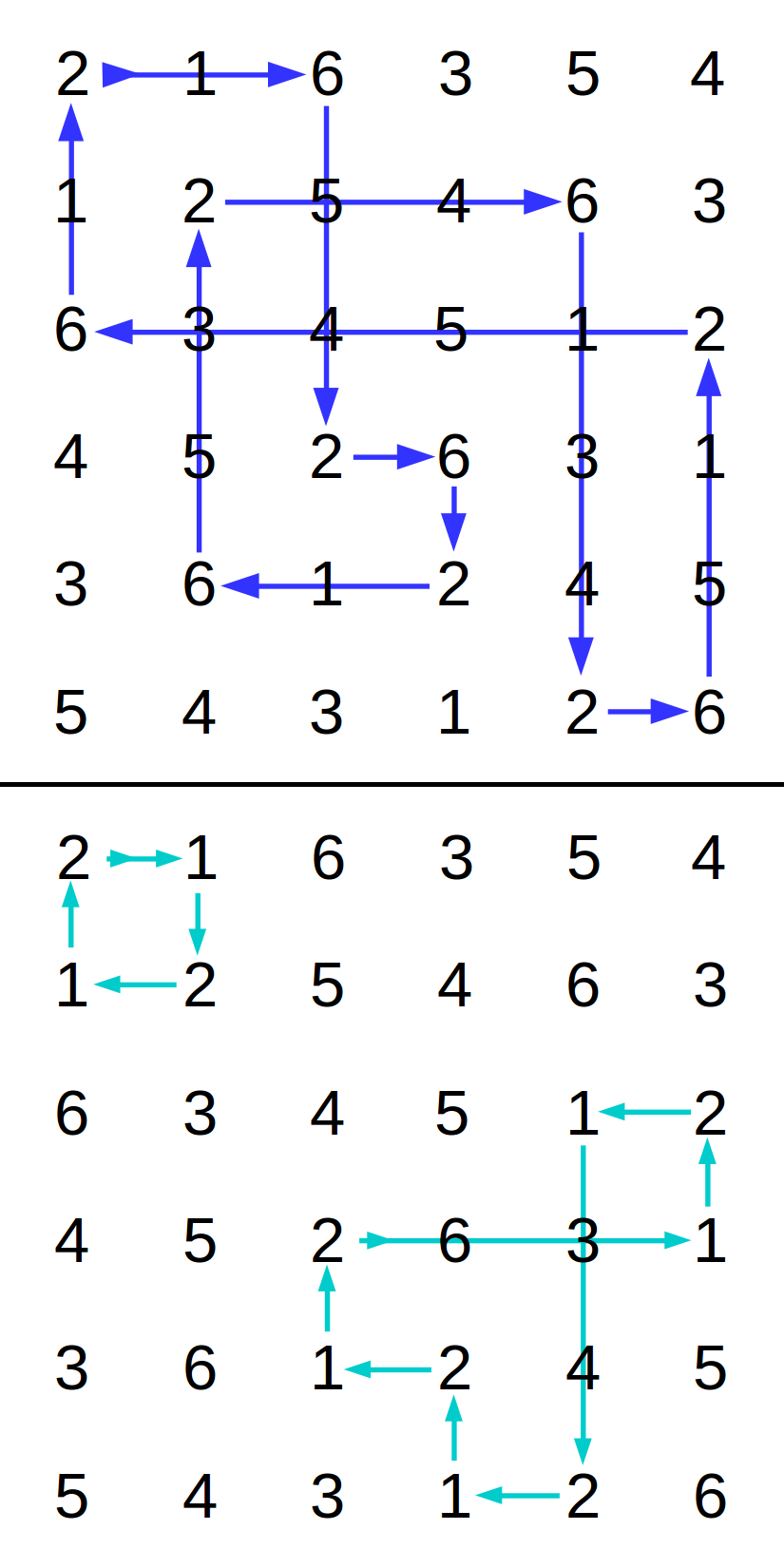
Figure 1 - Circuit paths in a Latin square
In a two-colored graph from a Latin Square, it is possible to trace from a cell containing one symbol to a cell with another symbol along a row-colored link, arriving at a different column, and then trace along a column-colored link from that location to a cell in a new row containing the first symbol. Continuing this process, from cell to cell with alternating symbols, identifies a path along links of alternating colors. This relationship induced by two symbols is called a matching. Because there are only two node colors, one for each symbol, it is a two-color matching. Because the link colors alternate in a strict row color and column color sequence, it is a two-color rainbow matching. [2]
A two-color matching in a Latin Square can be represented by a graph in which the node weights are always 2. This satisfies sufficient conditions, dating back to the Carl Hierholzer proofs regarding solutions to Euler's classic "Bridges of Königsberg" problem [8], for existence of a cyclic path along graph edges that connect the nodes in the matching. If the graph is connected, then there is a single path that forms a loop. Figure 1 illustrates some paths that can be traced within a Latin square along two different symbol matchings. Note that it is possible for a traced path to reach every row and every column, and when this happens the graph representing the matching is connected. However, it is seen that a path in another matching in the same Latin Square can return to the initial row-column location before all rows and columns have been visited. In this case, the two-color matching partitions the nodes into a set of isolated subgraphs — i.e., not connected. Each of those subgraphs is connected and forms its own closed cycle.
To simplify terminology, this paper calls the process of path-following along edges from node to node in a two-color matching tracing a circuit, analogous to tracing the flow of electricity through an electrical circuit. A loop identified by this tracing process is accordingly called a circuit. Define circuit length to be the number of distinct rows (or equivalently, the number of distinct columns) reached while tracing a circuit. If the length of the circuit equals N, the matching is connected, and the circuit is called a circuit of maximal length. Keep in mind that this terminology does not imply any kind of novelty.
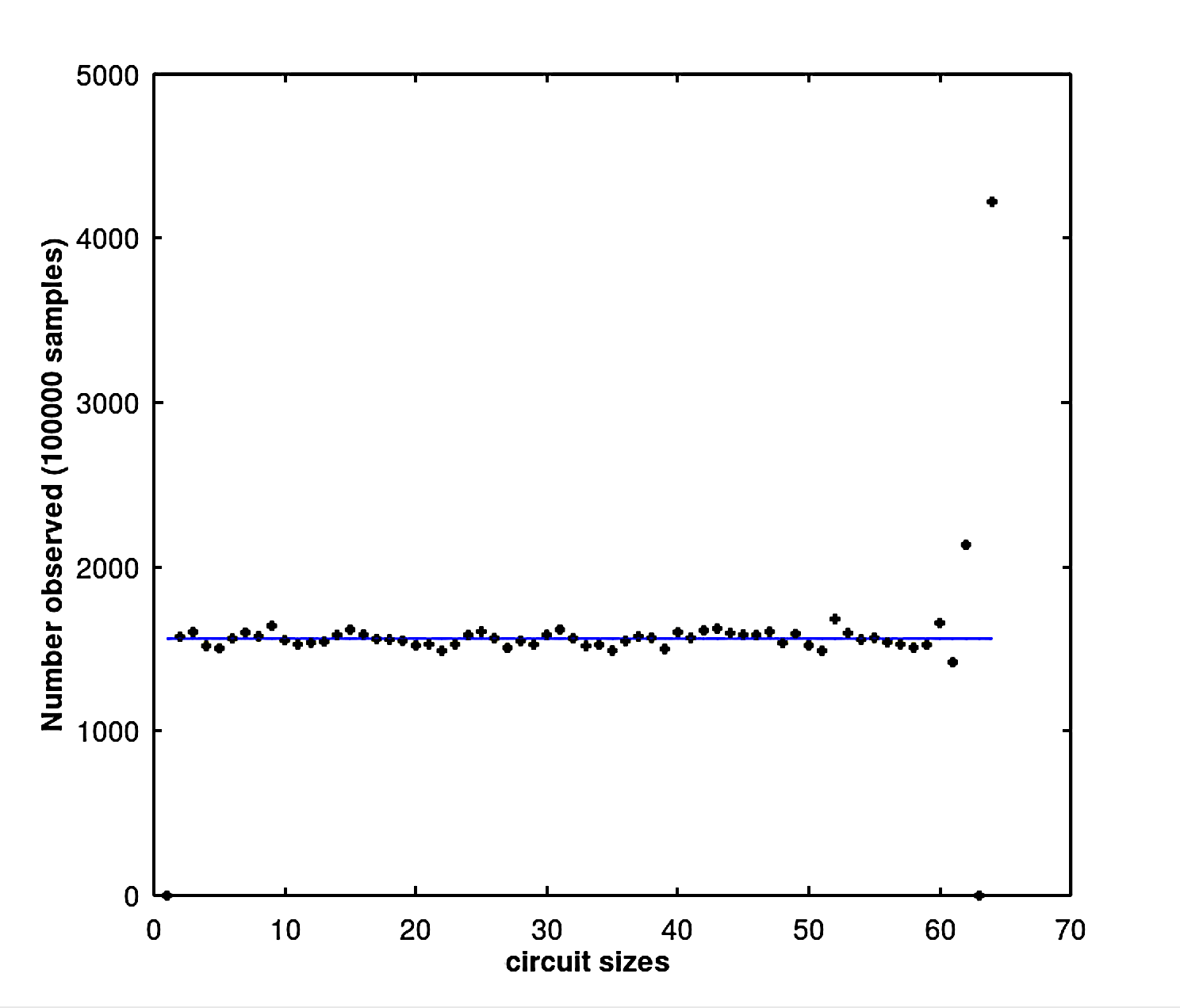
Figure 2 - Histogram of circuit lengths
Suppose that a Latin Square is selected at random from the set LS{N} of all possible Latin Squares of size NxN. From this Square, a pair of distinct symbols is selected in an arbitrary row, and starting with these, a circuit is traced along the implied two-color matching. How likely is it that the randomly-selected circuit turns out to have maximal length? For an empirical preview, consider the histogram shown in Figure 2. This shows the sizes of circuits observed from a sampling experiment in which 100000 Latin Squares are randomly obtained and tested. It can be seen that there are no circuits of size 1 — they cannot happen, because there are no "transition to self" nodes present in the graph of a rainbow matching. It can also be seen that there are no circuits of size of N-1, because that would require partitioning the nodes such that one node connects only to itself, which we just observed can never happen. In most other respects, the histogram looks like a uniform probability density distribution, except for what seems to be an anomaly for the longest circuit lengths. As we will show, this is actually a special property of this distribution, not an anomaly.
Label Matchings and Derangements
A derangement is a kind of permutation for which no element is allowed to remain in the place that it was previously. These structures have received some intensive study.[3] There are some important relationships to the internal structures of Latin Squares.
Construct a row transition list with its N locations initially empty. To populate this list according to a given Latin Square, select a first symbol and a second symbol for a mapping. For each row, observe within that row of the Latin Square the column where the second symbol is located. Record the column index in the row transition list: "for row j the second symbolcell was found at column k." Do this for every row. In a similar manner, a column transition list can be constructed by observing in each column the row location where the first symbol is located.
The transition lists can be used alternately to locate the cells that lie along a path within the two-colored matching graph representation. Consequently, we have an 2 x N structure that represents a two-color matching within the N x N Latin Square layout.
We do not lose or alter any information in the transition lists if we permute both transition lists in an identical manner. If this is done in such a way that the symbols in the column transition list are in collating order 1 through N, the ordered sequence is implicit and can be disregarded. What remains can then be interpreted: "if we were previously at row j, then column j of the transition list tells us the row where we arrive next as we trace a circuit within a matching." Since transitions do not start and end at the same location, the transition list is a derangement of 1 through N. If there is a cyclic structure within the derangement, it will correspond to a cyclic structure in the two-color matching from which the list was derived.
For studying properties of derangements, and thereby the two-color matchings, Algorithm 1 presents a simple rejection method to constructing derangement vectors randomly. (There is no particular reason for Algorithm 1 to prefer recording the positions of columns rather than positions of rows — either way produces similar results.) A two-color matching can then be constructed within an empty Latin Square layout using Algorithm 2, which traces alternately through the row transitions and column transitions indicated by the two lists. The significance of Algorithm 2 is that it can be followed in reverse to trace a matching and generate (or regenerate) the two transition lists. This demonstrates that, for purposes of enumeration, there is no distinction between counting circuits in a two-color matching and counting cyclic patterns within a derangement.
Algorithm 3 is particularly useful. It can be used to test for maximal circuits in any given Latin Square structure. If Algorithm 3 returns a count less than N, there is no cycle of maximal length for the specified two-symbol matching, nor a maximal cycle in the derangement structure representing it. It is sufficient to choose the start cell locations from the first row of a Latin Square, since a maximal circuit must visit the first row eventually, and any symbol pair that generates a less-than-maximal circuit starting from the first row cannot produce a maximal circuit from the remaining rows.
Counting cycles and circuits via derangements
Algorithm 1 can be modified so that once a cell location has been filled, no future choices can return to that location until all other assignments have been made. This forces construction of a cycle of maximal length. Examining the details of this modified algorithm reveals the following.
Theorem 1 The number of ways M(N) to construct a derangement with a maximal cycle length N is (N-1)! . The number of ways M(N) to obtain a circuit of a maximal size in a two-symbol matching of size N is (N-1)! .
This can also be verified experimentally by explicitly enumerating all possible derangements of a vector and counting the number of maximal cycles encountered.
Adapting algorithm 1 to count all possible derangements of a list of a given size is more complicated. A matching that is not connected might be partitioned into several disjoint circuits. So a different strategy is considered.
Suppose that the number of possible derangements of a list of length N is DN, and is known. Suppose that the number of possible derangements for a list of length N-1 is also known, and equals DN-1. We want to see if this information is sufficient to determine the number of possible derangements DN+1 for a list one element longer. There are two available strategies, as illustrated in Figure 3.
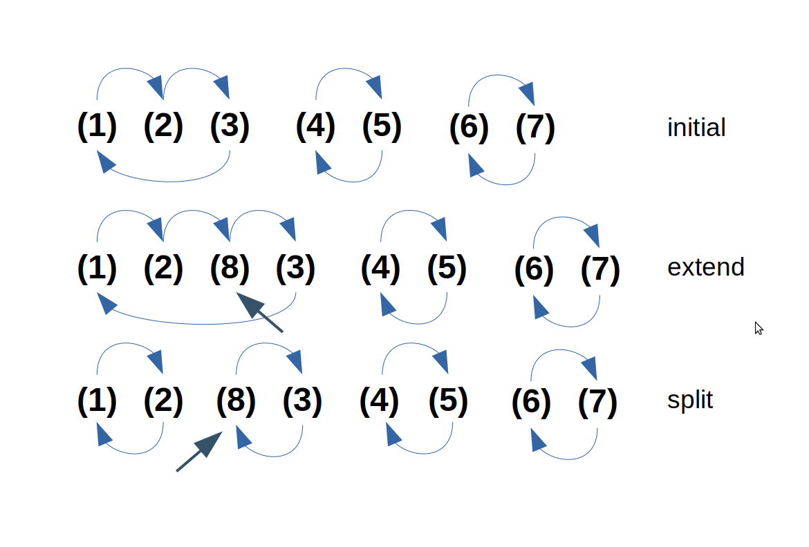
Figure 3 - Strategies for longer derangements
By extension. We can't introduce a new symbol in isolation, because a circuit must be length 2 or greater. To introduce a new symbol into existing derangements of N symbols, the new symbol N+1 must be spliced into a circuit that already exists in a derangement of size N. Given any initial derangement of N symbols, there are N locations available for insertion of a new symbol, immediately following one of the N symbols previously present in the initial derangement. Injecting the new symbol in this manner lengthens exactly one of the cycles from that initial derangement, never increases the number of cycles, and never produces a new cycle of length 2. Noting that the extension process can start with any of the DN derangements of the initial list of N symbols, this strategy provides N · DN ways of producing new derangements of length N+1.
By splitting. Start with a list of N symbols. Select one of these symbols and separate it from the others. We can now introduce a new symbol N+1 by pairing it with the previously isolated symbol to form a new cycle of length two. We know that for the remaining N-1 symbols in the list, there are DN-1 possible derangements. Appending the new two-length cycle to one of these derangements yields a distinct new derangement of N+1 symbols. Thus, there are N · DN-1 ways to obtain a length N+1 derangement using this strategy. It is not possible for the new length-2 cycle to arise using the extension strategy. Thus derangements produced by this strategy and by the extension strategy are disjoint.
There are no cases that are not covered by one of these two strategies. Combining the strategies yields Theorem 2.
Theorem 2 The number of derangements possible for a list of N symbols DN satisfies the recurrence formula
This relationship can be verified using integer induction and straightforward algebra, using start values D1 = 0 (there are no possible derangements for a single item) and D2 = 1 (there is only one way to swap a set of 2 items). TABLE 1 lists the first few terms of the D sequence. Correctness of the DN values can also be verified experimentally by systematically generating and counting all possible derangements of an arbitrary initial list.
   TABLE 1 -  Number of possible derangements of N symbols

    N         D(N)

     1        [0]
     2         1
     3         2
     4         9
     5         44
     6         265
     7         1854
     8         14833
     9         133496
     10        1334961
     11        16153027
     12        209855856
     ...
Probability of maximal circuits in derangements
If a derangement is generated at random, the probability P(N) that it contains a cycle of maximal length is given by the ratio M(N) / DN, where M(N) is given by Theorem 1 and DN is given by Theorem 2. TABLE 2 expands upon TABLE 1 to show the first few of these exact probability values. For verification, a Monte Carlo random experiment observed 10 million instances of artificial derangements, as generated by Algorithm 1, and counted how many of them had a maximal cycle. The results from this sampling experiment closely match the theoretical distribution, as shown in TABLE 2.
       TABLE 2   -  Probability of maximal derangement cycles

    N       M(N)          DN          P(N)             Monte Carlo test
            = (N-1)!                  = M(N) / DN
    0
    1         1           [0]           -------           -------
    2         1            1            -------           -------
    3         2            2            1.00000           -------
    4         6            9            0.66667           -------
    5         24           44           0.54545           -------
    6         120          265          0.45283           0.45319
    7         720          1854         0.38835           0.38844
    8         5040         14833        0.33978           0.33979
    9         40320        133496       0.30203           0.30186
    10        362880       1334961      0.27183           0.27175
    11        3628800      14684570     0.24711           0.24723
    12        39916800     176214841    0.22652           0.22634
    ...
The D(N) sequence grows slightly faster than the factorial M(N), as the P(N) ratio is seen to converge slowly and monotonically toward zero. To examine this more closely, consider the following sequence. The motivation for this will soon become apparent.
TABLE 3 displays the first few terms of F.
       TABLE 3 - First terms of sequence F(N)

 N       N!      1 / N!     D(N)    D(N)/N!       F(N)

 1       1        1         [0]      0            -1
 2       2        1/2       [1]      1/2           1/2
 3       6        1/6       2        1/3          -1/6
 4       24       1/24      9        3/8           1/24
 5       120      1/120     44       11/30        -1/120
 6       720      1/720     265      53/144        1/720
 7       5040     1/5040    1854     103/280      -1/5040
 8       40320    1/40320   14833    2119/5760     1/40320
    ...
We can observe from TABLE 3 that the first few F(N) terms satisfy
Suppose that the observed pattern holds for all integers up to some
positive integer N. Multiply by
-1 /(N+1).
Recast Theorem 2 into following form.
Substituting into the previous expression yields
Integer induction then leads to Lemma 1.
Lemma 1
for all positive integers N.
Next, these F terms are summed. At each step of the summation, one of the D terms cancels out a term from the previous partial sum. At the end, only two D terms remain; and one of these is D1 which can be dropped because it equals zero. This leads to Lemma 2.
Lemma 2
The series on the left side can be observed to be a partial McLaurin power series expansion for ex, evaluated at x = -1, except that the first two terms are missing. However, these two terms happen to have canceling values 1 and -1, contributing zero. That leads to the following modification of Lemma 2.
Lemma 3
Finally, combine Lemma 3 with the exact probability P(N) = F(N) / DN of a maximal-length circuit in a derangement, as displayed in TABLE 2. Simple algebra produces the main theoretical result.
Theorem 3
As N becomes large, the probability P(N) that a randomly-selected derangement of N terms has a cycle of maximal length converges to
Notice that the value P(N) would have been 1/N in an ordinary uniform distribution. This explains the "anomalous" probability observed at the end of the histogram in Figure 2.
TABLE 4 compares the first few actual values of P(N) to the asymptotic limiting curve provided by Theorem 3. The convergence is complete, for practical purposes, at about N=9. For verification, a Monte Carlo test applied to populations of 10 million random derangements confirms the theoretical result.
   TABLE 4 -- Convergence of probability for a maximal derangement cycle

    N        P(N)        Asymptote       Monte Carlo test
                        (Theorem 3)
    0
    1         -------      -------          -------
    2         -------      -------          -------
    3         1.00000      0.90609          -------
    4         0.66667      0.67957          -------
    5         0.54545      0.54366          -------
    6         0.45283      0.45305          0.45319
    7         0.38835      0.38833          0.38844
    8         0.33978      0.33979          0.33979
    9         0.30203      0.30203          0.30186
    10        0.27183      0.27183          0.27175
    11        0.24712      0.24712          0.24723
    12        0.22652      0.22652          0.22634
    13        0.20910      0.20910          0.20912
    ...
Probability of Maximal Circuits in Latin Squares
While the derangement theory provides much valuable insight, it is not the complete story for the case of Latin Squares.
Suppose that a Latin Square is to be constructed "randomly" one row at a time. The only constraint on the first row is that each of the N symbols must be assigned. Clearly, assignments for the first row are equivalent to an elementary random sampling from a set of N distinct symbols without replacement.
For filling the second row, the symbols can again be placed randomly, but subject to an additional derangement constraint so that no second row symbol can be placed in a column where that symbol already appears in the first row. Instead of N! ways of placing filling the second row, there are (N-1)! ways, by Theorem 1. This derangement constraint enforces the Latin property of Latin Squares, that no symbol can appear twice in any column.
For filling a third row, each symbol must satisfy additional derangement constraints: the new row must be a derangement of both of the preceding rows. Similarly, a fourth row must be a pairwise derangement of each of the three rows that preceded it, and so forth.
Figure 4
Two partial Latin Squares of size 6x6
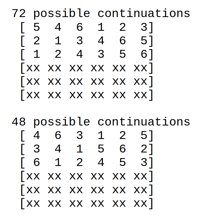
Consider for example the two partial layouts illustrated in Figure 4. Each one is a partial Latin Squares with 3 of the 6 rows assigned symbols, and with the remaining cells being empty. The number of ways to complete a Latin Square are counted comprehensively from these starting conditions, using a modification to Algorithm 4. We find that there are 72 possible completions starting from the first set of assignments, and 48 possible completions after starting from the second. In other words, the number of ways to satisfy the derangement constraints is dependent on which particular symbol assignment choices were made previously. With a sequence of "unfortunate choices," the derangement constraints can lead to a situation that zero choices remain available for configuring the next row — and then we have encountered the classic Latin Square completion problem.[4]
For Latin Squares that are small enough, it is feasible to simply generate the entire collection of all possible Latin Squares exhaustively, using a depth-first search strategy, counting and testing all of the completed Latin Squares so generated to find how many maximal-length circuits are present. As with unconstrained two-symbol matchings, the number of circuits counted in the Latin Squares, divided by the total number of circuits analyzed, yields the probability of encountering a maximal-length circuit at random, as displayed in TABLE 5. This is compared to the exact formula for derangement given by Theorem 2 and the asymptotic formula for derangements as given by Theorem 3.
   TABLE 5 -
   Comparing probability of encountering a maximal cycle in a
     derangement or a Latin Square (using exact enumeration)

  Size   Derangement   Derangement         Exact Latin Square
         Probability   Asymptote              Probability

    2     1.0000        -------
    3     1.000         0.90609                1.00
    4     0.66667       0.67957                0.50000
    5     0.54540       0.54366                0.64286
    6     0.45296       0.45305                0.42857
    7     0.38835       0.38833                0.38758
    8     0.33978       -------
    ...
It is apparent that the number of maximal cycles occurring in derangements and in Latin Square matchings are not the same. However, these two counts converge converges rapidly as N increases. That this should occur has already been posed as a formal conjecture by Cavenagh, Greenhill and Wanless,[3] that two rows of a Latin Square and a random derangement have asymptotically the same distribution. The relationship between derangements and circuit cycles lends empirical evidence to support that idea.
For statistical confidence, it would be desirable to extend the exhaustive counting approach for another couple of levels, but for Latin Square sizes larger than 7, the effort to generate and test all Latin Squares comprehensively starts to become prohibitive.
To obtain a reasonable empirical view of what happens in large Latin Squares, the testing method of Algorithm 3 is applied to sample sets of (at least) 100 million Latin Squares. The Latin Squares are obtained using Algorithm 4, except that the recursion is artificially terminated after identifying and testing 10000 Latin Squares; then Algorithm 4 is restarted, with the search order for the depth-first search randomly shuffled. Each depth-first search process recursively explores the local area where a Latin Square is found, seeking other "nearby" Latin Squares. This process of randomized depth-first searches and repeated restarts continues until the desired population of Latin Squares is obtained and tested. TABLE 6, extending TABLE 5, shows that estimates provided by the sampling and searching experiment correspond closely to the exact enumeration method for small Latin Squares, and also correspond to the asymptotic probability values provided by derangement theory for larger squares.
   TABLE 6 - Comparing probability of encountering maximal circuits
      in derangements and in enumerated Latin Squares

  Size N   Derangement   All Latin     Randomized   Sample size
           Asymptote     Squares       Sampling
    2       1.0000       1.00
    3       1.000        1.00
    4       0.66667      0.500000
    5       0.54540      0.642857      0.64272      1.0·108
    6       0.45296      0.428571      0.42758      1.0·108
    7       0.38836      0.387579      0.38623      1.0·108
    8       0.33994                    0.33992      2.5·108
    9       0.30209                    0.30266      2.5·108
   10       0.27165                    0.27211      2.5·108
   11       0.24716                    0.24774      1.0·108
   12       0.22664                    0.22699      1.0·108
   ...
Given the consistency of these probability estimates, TABLE 7 consolidates the information from the exact and asymptotic probabilities to produce a reference standard for values of the probability of encountering maximal circuits in randomly-sampled Latin Squares, with error less than ±0.001 .
  TABLE 7  - Reference probability of maximal-length circuits
                 in random Latin Squares

  Size          ref probability that a
    N             circuit is maximal

    2               1.0000
    3               1.0000
    4               0.5000
    5               0.6429
    6               0.4286
    7               0.3876
    8               0.3399
    9               0.3021
   10               0.2717
   11               0.2472
   12               0.2266
   N>12              e/N
Extending to a test procedure
While TABLE 7 is not theoretically satisfying, a fully-developed theory is not needed to obtain useful results.
The testing method is essentially an elementary test for equality of means. While formal and sophisticated statistical tests could certainly be designed, the goal is easy application and a very high degree of confidence in the test results. Theorem 4 indicates that the probability of obtaining a circuit of maximal length N in in randomly selected Latin Squares is closely approximated by p = e/N. Correspondingly, the probability of encountering any other non-maximal circuit length is q = (N-e)/N. The well-known Bernoulli distribution describes the distribution of repeated sampling experiments with two possible outcomes [6]. This distribution has the properties:
        expected value  =  p
        variance value  =  p q.
Appealing to the Central Limit Theorem [7], when this distribution is randomly sampled a very large number of times M, and the mean of the sampled population is estimated from these samples, the distribution of the estimates will have the properties
        expected value of estimate =  p
        variance value of estimate =  p q / M.
A confidence interval of 8σ and a test population of 1 million samples is suggested for this estimate, yielding a confidence of approximately 99.99999%. Interval sizes that correspond to the 8σ level are tabulated in TABLE 8, based on the "reference" probability values given in TABLE 7.
  TABLE 8  - 8 σ confidence interval for sample populations of
      M = 1 Million randomly sampled Latin Squares

  Size    ref probability p      8σ confidence interval
    N     of  maximal circuit

    4          0.5000                 0.004000
    5          0.6429                 0.003833
    6          0.4286                 0.003959
    7          0.3876                 0.003894
    8          0.3399                 0.003786
    9          0.3021                 0.003673
   10          0.2717                 0.003559
   11          0.2472                 0.003452
   12          0.2266                 0.003349
   N>12         e/N               8 * sqrt( (e/N * (1 - e/N))/M )
To summarize, the simplified test is performed as follows:
- Obtain 1 million Latin Squares produced by the generator under test.
- Apply Algorithm 3 to detect maximal circuits in each generated Latin Square.
- Count the number of circuits tested and maximal circuits found.
- Calculate the ratio of maximal circuits to circuits tested.
- If the resulting test statistic differs from the reference probability by more than the confidence level shown in TABLE 8, conclude that the generator under test does not produce random Latin Squares.
As a screening test, note that this is a necessary but not sufficient condition for randomness — failure of this test to detect a bias does not guarantee an unbiased generation process. As an extreme example, consider a generator algorithm that returns exactly the same Latin Square every time, one that happens to have a number of maximal circuits close to the expected number for truly random Latin Squares. The test would not report a problem -- despite the decidedly non-random generation strategy.
Application to randomness testing
As a practical demonstration, the suggested testing method is applied to the well-known Jacobson-Matthews (J-M) algorithm[3] . That particular algorithm does not really generate a new randomized Latin Square: it shuffles an existing one, (hopefully) breaking and restoring internal structures on a local scale so that global randomness results. There are two kinds of moves, a "proper" flavor that leaves the Latin Square with Latin Properties temporarily violated, and an "improper" flavor that can restore the Latin Properties. This is an iterative method, lacking a well-defined number of operations to guarantee statistical quality of the results. The iterative process is bounded, but in practice, consistency is restored much faster than the absolute bounds suggest. Any time the Latin Square layout is consistent, and Latin properties are restored, the scrambling process can be terminated, hopefully leaving a new and well-randomized Latin Square.
To test the J-M method, the following strategy was employed to estimate number of moves to apply. Two artificial initial patterns were selected, one exhibiting a deliberate over-abundance of maximal cycles, the other exhibiting a scarcity of them. The J-M algorithm is applied for the two starting patterns. The number of maximal circuits is tested at regular intervals, to watch the changing counts of maximal circuits until the probability estimates converge to the same number from both starting points. This number of moves was deemed adequate for purposes of this testing. For each size, a sample population of 10 million Latin Square results was generated by the J-M method and tested for the presence of maximal circuits. The results are shown in TABLE 9, along with the number of moves employed.
  TABLE 9  -  Tests of the Jacobson-Matthews generator

  Size  Reference    Tested        Moves     Difference   % Excess max
        probability  probability   applied                  circuits

    5     0.64286    0.6552         12        0.0122         1.9
                     0.6550
    6     0.42857    0.4513         16        0.0228         5.3
                     0.4514
    7     0.38758    0.3963         32        0.0086         2.2
                     0.3960
    8     0.33994    0.3439         90        0.0039         1.2
                     0.3437
    9     0.30209    0.3051         110       0.0029         1.0
                     0.3049
   10     0.27165    0.2735         150       0.0021         0.8
                     0.2738
   11     0.24716    0.2489         160       0.0016         0.7
                     0.2487
   12     0.22664    0.2272         140       0.0006         0.3
                     0.2271
Using the simplified test of TABLE 8, the testing indicates the presence of biases favoring more than the expected number of maximal-length circuits when the generated squares are size 8x8 or less. The results are inconclusive for squares that are larger. A more formal and rigorous statistical test, using a larger sample set, could be expected to detect observable bias through a larger range. These biases are real, but depending on the application, all of them might be considered too small to matter. A point of theoretical concern, however, is that the Jacobson and Mathhews method is generally believed to convergence to randomness for any size Latin Square after a large number of algorithm "moves" — see for example the introductory discussion in [3]. The testing here indicates that the results converge to randomness only when Latin Square sizes become large.
Conclusions
A straightforward method for checking the randomness of Latin Squares produced by a pseudo-random generator has been presented. While the idea is based on established theory regarding derangements, the extension to Latin Squares remains empirical, and theoretical work is needed.
The simplified test is easy to perform, and the results are easy to interpret. There is a long history of applying this kind of empirical testing for evaluating the quality of real-valued pseudo-random variate generators [9], and similar utility can be expected for the testing of pseudo-random Latin Square generators.
The supporting theory presented here applies an interesting and perhaps previously unknown property of the probability distribution of circuit sizes in the two-symbol matching structures within Latin Squares. While this distribution superficially looks uniform, we have shown that this is illusory. The only distribution term definitively known at this time is the probability that an arbitrarily selected circuit has maximal length. Fully characterizing all of the other distribution terms, first for derangements, and beyond that for rows/columns of Latin Squares, remains a topic for study.
Further study of the "mutual pair-wise derangement relationships" among Latin Square rows might lead to new insights about the nature of Latin Squares and Latin Square completion problems.
If a generator algorithm consistently produces Latin Squares that have an unexpected number of maximal-length circuits, that is strong evidence that the results of the generator algorithm are not random. The popular Jacobson-Matthews algorithm was chosen to demonstrate this criterion, and its bias is clearly detected in smaller Latin Squares. However, the bias is small, and becomes smaller for Squares that are larger. This might be interpreted either as evidence for or against the algorithm's application, depending on application requirements.
Appendix: Algorithms
A simple rejection method to construct derangement vectors randomly. Every possible derangement is equally likely to be produced.
    Algorithm 1: Construct a uniformly random derangement

Construct an "available labels" list of length N.
   Initialize it with with index numbers 1 through N
Construct a "deranged" list of length N.
   Initialize it with all cells empty.

Repeat
  For each row location j from 1 through N-1 :
     Remove label j from the available labels list
     Select label k randomly from the remaining available labels
     Remove label k from the available list
     Save k at location j in the deranged list
     Replace label j in the available labels list
  End For

  Take the last label item from the available list
  If it is not equal to N,
     Save the last label in deranged list location N
     Exit the Repeat loop
  Else
     Copy all labels back to the available labels list to restart
  End if
End Repeat
A method to map any arbitrary pair of deranged symbol lists into a matching in a partial Latin Square layout.
    Algorithm 2: Construct random two-label matching from derangements

Construct an NxN layout of a Latin Square
Leave all layout cells initially empty
Obtain the row and column derangement indexing lists
Obtain the row label and column label symbols

Repeat:
  Arbitrarily select a start row index from the row list
  Remove the start row index from the row derangement list
  Set the current row index equal to the start row index

  Repeat:
    Extract the value colx from the row derangement list
       at the current row index location
    Remove from the row derangement list the item present at current row index
    Set the current column index to colx
    Set the column label into the Latin Square cell
       at location (current row, current column)
    Extract the value rowx from the column derangement list
       at the current column index location
    Remove from the column derangement list the item present at current column index
    Set the current row index to rowx
    Set the row label into the Latin Square cell
       at location (current row, current column)
    If the current row index is the sames as the start row index
       Exit the inner Repeat loop
    End If
  End Repeat

  Increment the partition count
  If no items remain in the row derangement list
    Exit the outer Repeat loop
  End If

End Repeat
A method to test whether an arbitrary circuit found in a Latin Square has maximal length.
    Algorithm 3: Test a two-symbol matching for a maximal cycle

Obtain the Latin Square layout to test.
Locate the start row for the cycle under test.
Obtain the first symbol and second symbol to use for
   generating the matching.
Let the start cell be the cell in the first row containing
   the first symbol.
Set current row equal to start row.
Length count = 0
Repeat:
  Find column index of second symbol in current row.
  Set current column equal to located column index
  Find row index of first symbol in current column.
  Set current row to located row index
  Increment circuit length count
  If the current row index equals the start row index,
     Exit the repeat loop
End repeat

Report the circuit length detected
Depth-first randomized search to construct and count small Latin Squares combinatorially. (Note: N2 levels of recursion! This is impractical for large squares.)
    Algorithm 4: Systematically construct and count Latin Squares

Initialize:
  Set all N x N cells of Latin Square empty
  Construct an ordered list of symbols ALL = {1 ... N}
  For each row
     Set available symbols list for row equal to ALL
  End for
  For each column
     Set available symbols list for column equal to ALL
  End for
  Set Latin Square count equal to 0

Recurse:
  If there are no empty Latin Square cells remaining:
     Increment Latin Square count by 1
     [ Apply desired testing to the completed Latin Square ]
     Return from recursion
  Select an empty Latin Square cell at random
  Observe the current cell's row and column
  Set available list for cell = symbols available in its row AND column
  If there are no symbols available for assignment:
     Return from recursion
  Shuffle cell's available list

  For each symbol in cell's available list
     Assign symbol to cell
     Remove symbol from row availability list
     Remove symbol from column availability list
       Recurse
     Clear symbol from cell
     Restore symbol to row availability list
     Restore symbol to column availability list

Report the count of Latin Squares obtained [tested]
References:
[1] Diestel, Reinhard, "Graph Theory"; 5th Edition (2016). Graduate Texts in Mathematics, Volume 173, Springer-Verlag; Heidelberg Graduate Texts in Mathematics, Volume 173.
[2] Gyárfás, András; Sárközy, Gábor N. "Rainbow matchings and cycle-free partial transversals of Latin squares"; Discrete Mathematics 327 (2014), 96–102.
[3] Cavenagh, Nicholas J.; Greenhill, Catherine; Wanless, Ian M., "The Cycle Structure of Two Rows in a Random Latin Square"; Wiley InterScience , DO1 10.1002/rsa.20216 (2007).
[4] Colbourn, C. J., "The complexity of completing partial Latin squares" (1984); Discrete Applied Mathematics 8(1), 25–30.
[5] Jacobson, M. T.; Matthews, P. "Generating uniformly distributed random Latin squares"; Journal of Combinatorial Designs 4 (6)" (1996), pp 405–437 .
[6] Evans, M.; Hastings, N.; and Peacock, B. "Bernoulli Distribution"; in Statistical Distributions, 3rd ed. (2000), Ch. 4 pp. 31-33.
[7] Montgomery, Douglas C.; Runger, George C. "Applied Statistics and Probability for Engineers", 6th ed. (2014), p. 241.
[8] Hierholzer, Carl; Chr. Wiener (1873). "Über die Möglichkeit, einen Linienzug ohne Wiederholung und ohne Unterbrechung zu umfahren". Mathematische Annalen" (1873) Ch 6 pp. 30–32.
[9] Knuth, Donald, "The Art of Computer Programming, Volume 2: Seminumerical Algorithms", Chapter 3, Addison-Wesley Publishing Company, 1969