A Better Jacobson-Matthews Latin Square Shuffler
Larry Trammell (retired)
August 30, 2023
version 1.0
Abstract
For the problem of obtaining a
Latin Square "randomly" — that is, every possible Latin Square has an
equal probability of being produced — the Jacobson/Matthews algorithm
has been the method of choice for decades; but it has a serious scaling problem.
It expands a Latin Square layout into an equivalent three-dimensional grid
where computations are performed, then projects final results back to a
two-dimensional layout. However, it is possible to dispense with the
expansion and projection processing, and perform the manipulations directly
in the original two-dimensional storage. Adding an appropriate termination
heuristic, and replacing the O(N) conflict searches with O(1) indexing,
offers an implementation with complexity O(N2) for expected
computational effort, yielding sufficient results.
Keywords: Latin Square, random sampling, algorithm, generator,
Jacobson-Matthews method, efficiency, termination, complexity
Background
The Jacobson-Matthews algorithm [1] shuffles the contents of a Latin Square to produce a new, randomized Latin Square, hoping that the end result is indistinguishable from a truly random Latin Square. If every possible Latin Square has precisely the same probability of being delivered by an algorithm, then that generator algorithm is random. If certain kinds of results are slightly more or less likely, the generator is biased. Bias is important but not necessarily a barrier to practical application; for example, computer-generated pseudo-random numbers, which are not completely random, are useful (with appropriate care) for highly demanding cryptographic applications.[2]
A Latin Square is a two-dimensional layout organized as N rows and N columns, where N is a specified configuration constant. Symbols from an ordered symbol set are placed into the N2 cells of the Latin Square layout, such that each of the N symbols is assigned exactly N times within the layout, and such that every symbol appears exactly one time in every row and exactly one time in every column. These restrictions on the number of symbols and where they appear are called the Latin constraints.
The Jacobson-Matthews algorithm doesn't really know how to establish a layout satisfying the Latin constraints. It only knows how to preserve those properties. This is one of its major drawbacks, and it means that it must be started from some kind of "canned" pattern that is already a Latin Square. A lot of the effort of the algorithm goes toward obliterating any observable correlation to the contents of that initial pattern.
There is an alternate representation for a Latin Square that the original presentation uses, in which the row index, the column index, and the symbol set are represented in a 3-dimensional grid. [3] Each node within this grid is uniquely identified by a triplet of coordinates: row index, column index, and symbol index. Every location is marked with one of two tokens — "empty" or "occupied. For example, if row 4, column 1 of the Latin Square layout contains the symbol "B" then the row-column-symbol grid location (4,1,"B") is marked as occupied.
The Jacobson-Matthews algorithm uses numeric code 0 to represent the unoccupied labels, implying empty, and numeric code 1 to represent occupied labels, indicating the row-column-symbol triplet represented by this location is present in the two-dimensional Latin Square representation. That label set is augmented to include one more special code: a −1, which can be interpreted as "negatively occupied." If a negatively occupied marking is applied to a grid location that is already marked occupied, the previous marking is obliterated and the node marking at that location is set to empty. Latin Square constraints can be recast in terms of the numeric labeling scheme by observing that the sum of all the label numbers along any line parallel to a row, column, or symbol axis is always exactly 1.
The Jacobson-Matthews algorithm uses a sub-structure based on two given grid triplets. Given pairs of distinct coordinates (x1,x2), (y1,y2), and (z1,z2), choosing one coordinate from each pair generates one of 8 different coordinate triplets. Triplets that differ in only one of the coordinate are called adjacent. Note that three of these triplets are adjacent to (x1,y1,z1) and three others are adjacent to (x2,y2,z2). This set of eight nodes define the corners of a rectangular prism sub-structure. To guarantee that Latin properties are not violated, there can be no more than 4 nodes in any such prism that are marked occupied.
Also observe that if a node (x1,y1,z1) is marked as "empty," then the Latin properties guarantee that (x2,y2,z2) can be found such that the adjacent nodes (x2,y1,z1), (x1,y2,z1) and (x1,y1,z2) are marked occupied. Basically, this is just saying that every symbol occurs in every row, every symbol occurs in every column, and every cell in the layout has a symbol assigned.
The Jacobson-Matthews shuffler proceeds by temporarily and locally relaxing Latin constraints. One extra occupied label is allowed in any grid position. However, to maintain the constraint that the sum of the row, column, and symbol markings is always 1, whenever there is an additional occupied marking, it must be balanced by a negatively occupied marking, so that the two cancel out of the sum. Only one anomalous negatively occupied marking is allowed in the grid at any time (so the structure does not degrade to chaos). The shuffling then proceeds by shifting the locations of the markings in a systematic manner within the current prism, subject to certain random choices, while maintaining the sum constraints. This process is repeated, over a large number of prisms, until the anomaly resolves itself, eliminating the negatively occupied marking, and leaving a correctly-structured grid.
Equivalence of representation
The expansion from the 3-dimensional grid is reversible. At any time, it can be projected down into the two dimensional Latin Square layout by locating the x,y coordinates of each cell, locating the z coordinate of the grid location marked as occupied, and storing the z coordinate as the label content within cell x,y.
However, when multiple markings project into the two-dimensional representation, information about the third dimension is lost, unless it is preserved separately. Since there is only one negatively occupied anomaly present at any one time, a small, fixed-size auxiliary storage area can keep all of that extra information. Meanwhile, the cells in the regular 2-dimensional Latin Square storage maintain all of the unambiguous information. Because the maintained information is exactly the same, the two structures are completely equivalent. There is no need to explicitly expand and use the theoretical three-dimensional grid.
Proper and Improper "moves"
The Jacobson-Matthews algorithm proceeds by applying certain controlled shifts to the positions and values of symbol locations. At first, all Latin constraints are satisfied, and the state is called proper. A move in a proper state applies certain label reassignments to the nodes in the current operating prism, and this can force a negatively occupied label into existence. The location where this anomalous label occurs is tracked in the algorithm state.
After that anomaly exists, the state of the grid is said to be improper. Moves are also applied to prism structures in the improper state, causing the anomalous negatively occupied label to shift to a different location, or causing its cancellation. When cancellation happens, all conflicts with the Latin constraints are resolved, and the storage layout once again becomes proper.
Each kind of move causes displacement of markings within grid storage as a side effect. The accumulation of these effects, spread across the layout over time, and controlled by uniformly random decisions along the way, results in an apparently random rearrangement of the symbols within the Latin Square storage.
Moves from a proper state
The Latin Square and corresponding grid always begin in a proper state, so this kind of move always happens first.
A move when in the proper state begins at an empty grid location called the start location, selected uniformly at random. From that start location perform line searches to determine the three adjacent nodes that are marked occupied. Next, the nodes other than the start node that are mutually adjacent to pairs of the three occupied nodes are located. The node that is mutually adjacent to all of those last three nodes forms the far diagonal corner of the rectangular prism. These nodes constitute the current prism on which the algorithm operates.
The nodes adjacent to the start node are occupied by construction. This leaves only one more location in the prism that could possibly be occupied: the one at the diagonal far corner.
Each move conforms to the following rules.
- If a node is marked empty and occupied is to be applied, replace the empty marker with the occupied marker.
- If a node is marked negatively occupied and occupied is to be applied, the two markers obliterate each other and the node is marked empty.
- If a node is marked occupied and empty is to be applied, replace the occupied marker with the empty marker.
- If a node is already marked empty and an additional empty is to be applied, the node is marked negatively occupied.
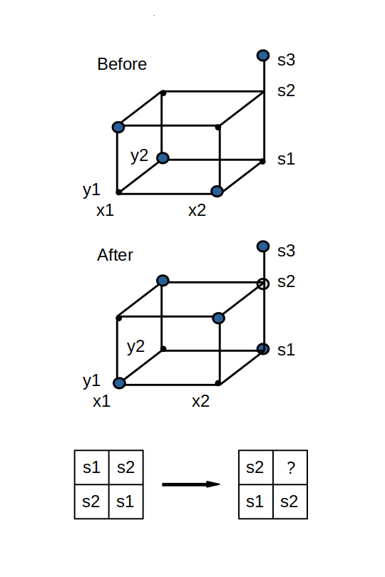
Figure 1 - Move in proper state
In Figure 1, the start node is located at (x1,y1,s2), and the far diagonal node for the prism is located at (x2,y2,s2). When a move is applied, it operates on the nodes in the selected prism by applying occupied at the start node, applying empty at the adjacent three nodes, applying occupied to the next three adjacent nodes, and applying empty to the diagonal node. The result is seen in the lower part of Figure 1. The move applies an equal number of filling and emptying operations in each row, in each column, for each symbol option, thus preserving the total number of nodes marked occupied along each dimension.
The outcome, however, is different depending on whether the diagonal node was originally marked occupied or empty. In Figure 1, if the diagonal node at (x2,y2,s2) had been marked occupied prior to the move, the final action of the move would set that node label to empty. No anomalous markings would be created and the grid remains in a proper state. But what happened in Figure 1 is that the (x2,y2,s2) node was initially marked empty, and the final action of the move assigned the label negatively occupied to that node. The node originally marked as occupied (not within the prism), and a node within the prism at (x2,y2,s1) set to occupied by the move, are also present along the same s-dimension line. As the node labels are summed along the s dimension, the -1 of the negatively occupied node cancels out a +1 value of one of the occupied nodes, so the total remains unchanged at 1.
When the grid is projected vertically downward onto the row-column two-dimensional layout of the Latin Square, an improper state presents a challenge. Symbols from two nodes marked occupied plus one symbol for the node marked negatively occupied will all project down to the same cell, producing a conflict. The conflict information is preserved separately, and the cell is considered unassigned.
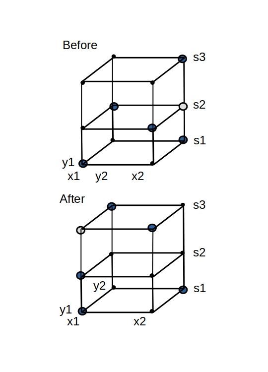
Figure 2 - Move in improper state
Moves from an improper state
The algorithm cannot terminate until the anomalous negatively occupied marking has been resolved, which can happen by applying moves while in the improper state.
Moves in an improper state always use the node having the anomalous negatively occupied marking as the start node. A line with a negatively occupied node means that there are two occupied nodes also along the same line. Locate them, and choose one of them uniformly at random. The same thing happens for row, column, and symbol. The conflicted start node and the three occupied adjacent nodes establish the new rectangular prism where the next move is applied.
The move in this new prism is the same as in a proper state, with one important differences. Applying an occupied marking to the negatively occupied start node obliterates the marking there, forcing it to empty. It can be seen in Figure 2 that the final operation at corner diagonal of the current prism could end up marked either empty or negatively occupied, depending on whether or not an occupied mark was there previously. If empty, then a negatively occupied marking results after completion of the move, and the state remains improper. If the diagonal node ends with an empty mark, the state becomes proper.
In the two dimensional projections, the moves are united by a common theme. Each move operation affects four cells forming the corners a rectangle. A move can "remove a label," "add a label," or "create a negative label." In a manner similar to the two-valued grid markings, a "label" and its "negative label" assigned to the same cell will annihilate each other. A move can leave a cell with multiple label assignments, a temporary violation of Latin constraints.
Let the cell that is the projection of the grid's start location be identified by coordinates x1,y1. Let the projection of the grid's far diagonal location be identified by coordinates x2, y2. Certain symbols A and B are selected, as detailed later. A move as seen in two dimensions then consists of the following operations:
- Remove symbol A from cell x1, y1
- Add symbol B into cell x1, y1
- Remove symbol B from cell x1, y2
- Add symbol A into cell x1, y2
- Remove symbol B from cell x2, y1
- Add symbol A into cell x2, y1
- Remove symbol A from cell x2, y2
- Add symbol B into cell x2, y2
Details of moves in a two-dimensional layout
The results of applying a move, as seen in two dimensions, will depend on the starting state, and the cells that are chosen for the current operating rectangle. This section catalogs and details all of the possibilities, so that correspondences between the two- and three-dimension representations are clear.
Case 1 : Starting from a proper state
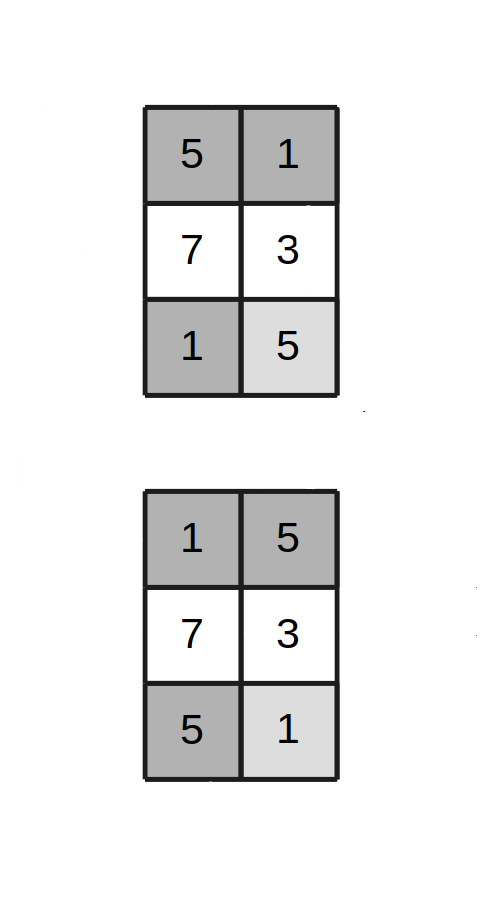
Figure 3, Case 1 - Move in proper state
Ends proper
Select any cell completely at random. Observe the symbol currently stored there. This will be "symbol A". In Figure 3, the start cell at the upper left is seen to contain the symbol 5.
Select any symbol other than A at random. This will be "symbol B." Since B is not the same as A, the symbol B will be located at two other adjacent cells. In Figure 3, these corner cells contain the selected symbol 1. These corner cells identify a second row and column to define the current rectangle. Locate the diagonal cell where the new row and column intersect. Let this be "symbol C".
Case 1 arises if it so happens that symbol C at that diagonal location matches symbol A from the start cell. After the move operation using symbols A and B, it can be seen in Figure 3 that the 1 symbols and 5 symbols have swapped places. The state remains proper.
Case 2 : Starting from a proper state

Figure 4, Case 2 - Move in proper state
Ends improper
Identify the cell locations and symbols exactly the same as in Case 1. But Case 2 arises if it so happens that symbol C at the diagonal location does not match symbol A from the start cell. In Figure 4, the symbol found there is 6.
After the move operation is completed, it can be seen that the A symbols went where the B symbols were previously, the B symbol replaces the A symbol, and there is a conflict at the diagonal location. As shown in Figure 4, the diagonal cell receives an additional A symbol, the C symbol remains there, and a negative-B symbol is added for the symbol that was removed but not present. The state is improper.
Case 3 : Starting from an improper state
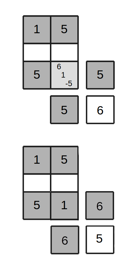
Figure 5, Case 3 - Move in improper state
Ends proper
The start cell is the one with the conflicts. The "negative symbol" present at that location means that there must be two "positive" copies of that symbol present somewhere in its row and column. Select one of these for the row and one for the column, uniformly randomly. These will be the two corner cells of the new operating rectangle. In figure 5, we can see that two new cells with symbol 5 were located.
In the new diagonal cell where the row and column of the selected corner cells intersect, examine the symbol present there. Case 3 arises if it so happens that the symbol at that location matches the symbol that was previously present at the current start cell. In figure 5, symbol 6 was found at the new diagonal cell. For this case, let symbol B be the symbol that is negative at the conflict cell, and let A be the remaining symbol there. Let A=1 and B=5.
Apply the move to the rectangle containing the start cell, the new diagonal cell, and the other two identified corner cells. The negative symbol at the start cell is canceled by one of the added symbols, and another symbol is canceled, leaving a single symbol present. At the completion of this move, as seen in Figure 5, the layout becomes proper again.
As the goal is "improvement," a liberty is taken here to deviate from the original algorithm. Observe that "move" operations are reversible. If both random selections for the new diagonal location happen to match the row and column used by the previous move, the new move "unwraps" the results of the previous move as if the pair of moves never happened. From an efficiency standpoint, there is no point in allowing such thrashing. From a theoretical standpoint, the existence of move-unmove infinite cycles undermines the claim that the move sequence is finite and bounded. Possibility of a bounded sequence is restored by insisting that at least one of the "random" selections must be a row or column that was not involved in the preceding move, assuring forward progress.
Case 4 : Starting from an improper state
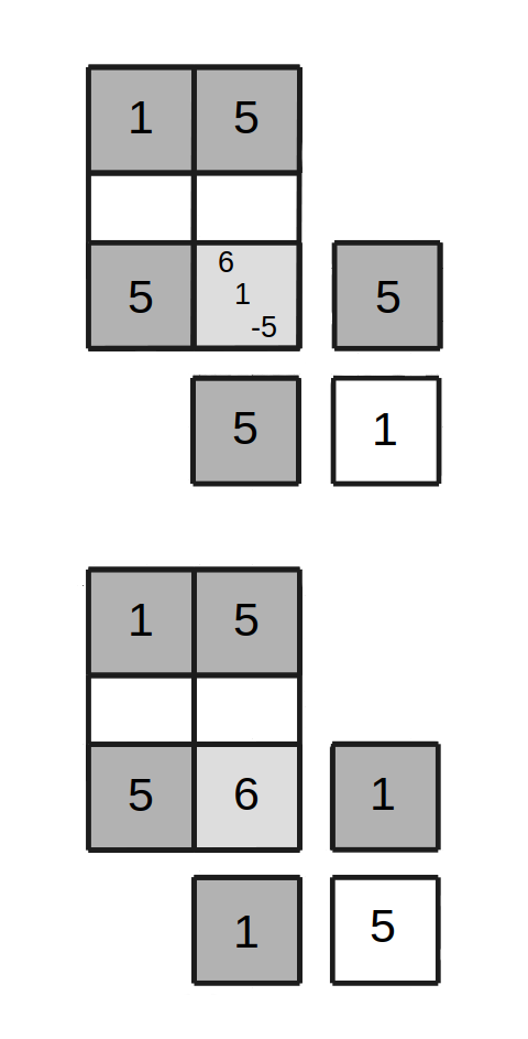
Figure 6, Case 4 - Move in improper state
Ends proper
This case proceeds exactly the same as Case 3, up to the point that the new diagonal symbol is observed. Case 4 arises when the symbol at that diagonal cell is found to match the other positive symbol associated with the conflicted start cell, not the one previously present in that cell. In Figure 6, the symbol at the new diagonal location is 1.
In this case, let symbol B be the symbol that is negative at the conflict cell, and let A be the symbol currently in the new diagonal cell. For Figure 6, A=1 and B=5. After the move, the layout is found to be proper, also as shown in Figure 6.
Case 5 : Starting from an improper state
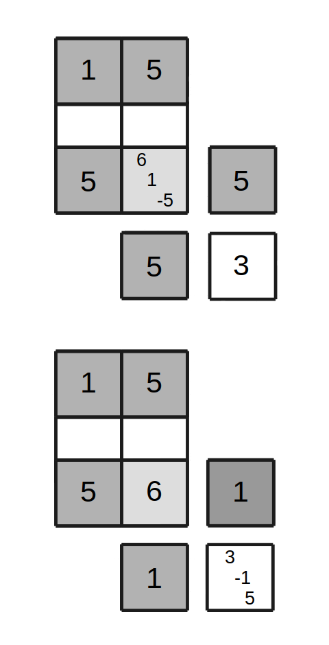
Figure 7, Case 5 - Move in improper state
Ends improper
This case proceeds exactly the same as Case 3 and Case 4, but when the new diagonal location is examined, neither Case 3 nor Case 4 applies. In Figure 7, the diagonal symbol turns out to be a 3.
Pick one of the two non-negative symbols associated with the conflict cell, uniformly at random, and use this as the A symbol. Let B be the value from the conflict cell that was negative. In the example of Figure 7, A=1 and B=5 were selected. After the move is applied, the conflict is resolved at the start cell, but reappears in the new diagonal cell, associated with a different trio of conflicting symbols. The state remains improper.
The 5 cases just detailed cover all possible situations, so it is only a matter of determining which one has happened, then following through the required processing for that case. Notice that each case makes some random choices. In the proper case, the choices determine the locations and symbols involved. In the improper case, the choices determine whether the conflict is resolved and, if the state is improper, where the next move will start.
Iterations and termination
While the algorithm is not fundamentally changed by its two-dimensional representation, the new view makes some of its properties easier to see. Here are some of these properties.
- The two states of the algorithm, proper and improper, are guided by probabilities that determine how often each kind of move operation is applied.
- The probabilities are nearly independent for cases starting in a proper state because locations and symbol choices are highly random, but even so, still constrained by Latin properties.
- The probabilities are more constrained for cases starting in an improper state, because some symbols, rows, and columns are shared from one improper move to the next.
- Each processing case directly determines whether a state change occurs or not.
- The probabilities are stationary, fixed by the constraints of the Latin Square.
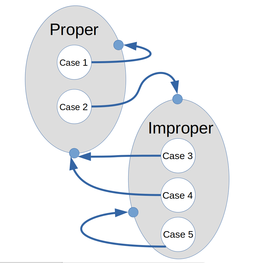
Figure 8 - A Markov-like model for state changes
Even though the structure does not fully satisfy the independence conditions for a Markov Chain representation, the structure is highly suggestive of one, as illustrated in Figure 8.
Taking an empirical approach, we might ask how often the algorithm reaches each of the illustrated states. Performing an experiment in which 2400 Latin Squares are generated for each Latin Square size, and 5 N2 moves are applied to each layout by the algorithm, we can count how many times each of the processing cases occurs. Table 1 shows the probabilities as a function of Latin Square size, as derived from this experiment.
  TABLE 1 -
  size N   moves applied       prob p             prob q
                           (becoming proper)  (becoming improper)
    10       504330            0.183974           0.816026
    12       725070            0.155350           0.844650
    16       1287161           0.117967           0.882033
    20       2010195           0.095479           0.904521
    25       3138290           0.077455           0.922545
    32       5136658           0.060520           0.939480
    42       8844061           0.046557           0.953443
    56       15711137          0.035127           0.964873
    74       27421535          0.026646           0.973354
    100      50058364          0.019797           0.980203
    128      81991279          0.015499           0.984501
Figure 9 shows the relationship between the size of the Latin Square and the probabilities (estimated) of being in a proper state. The best-fit line upon which the actual data are superimposed is
1/p ≈ 0.5 + 0.5 N
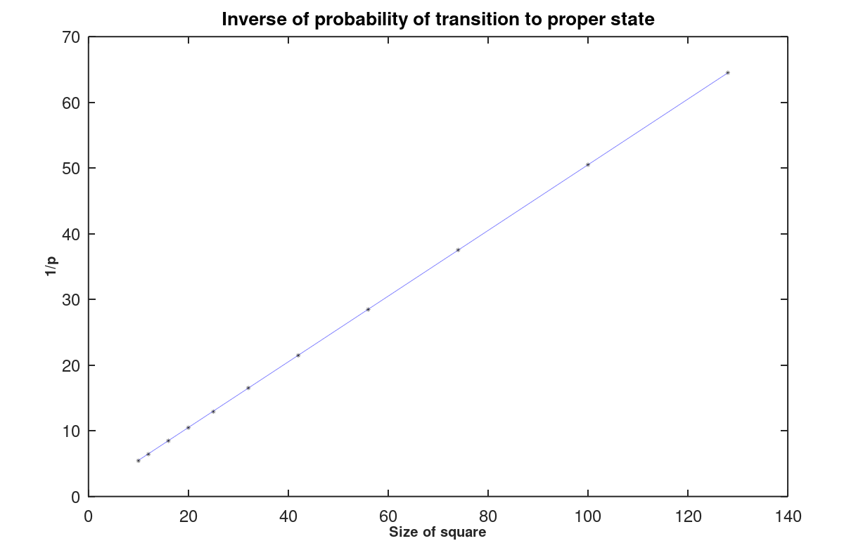
Figure 9 - Inverse of probability of proper state
The probability of being in a state relates directly to the probability of reaching that state. This is particularly relevant for transitions from an improper state to a proper one, because the algorithm cannot terminate until a proper state is reached. This might require no additional moves, if the state happened to be proper at the moment the minimum move count was reached. But much more often, the state is improper, and several moves will occur before returning to the proper state. How many?
With static probability p of arriving at a proper state, and a static probability of 1-p of staying in an improper state, this is similar to a geometric distribution, for which the expected number M of "independent trials" (additional moves) to reach a proper state is 1/p. This is an over-simplification, because the "trials" are not independent. Figure 10 shows the expected number of additional moves M. A least-squares best fit shows that to a good approximation
E(M) ≈ 0.5930 N - 2.1250
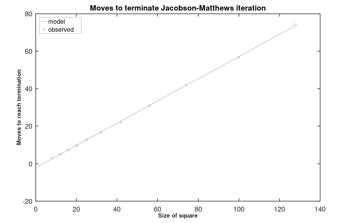
Figure 10 - Extra moves to termination
During the experiment, information was also collected about the variance of the counts of extra moves, as illustrated in Figure 11.
Stddev(M) ≈ √2.0 * E(M)
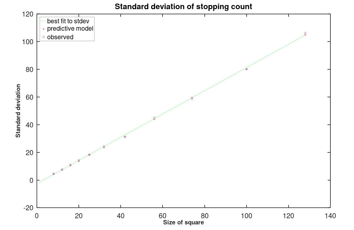
Figure 11 - Standard deviation of extra moves to termination
It is beyond the scope of this paper to explain why these distributions are the way they are. However, it is sufficient for now to note that the highly linear character of these curves indicate that the O(N3) bound provided by the original authors [1] does not appear to have much practical meaning for describing the terminal behavior.
Practical concerns about sufficiency
Each algorithm move affects four cells in a rectangular arrangement. If we make broad assumptions that these four cells selected are independent of each other, and that the label assignments in those cells could be anything, we might then attempt to describe the probability that a given cell is affected by any given move.
- p = 4 / (N2)
The probability of a cell being touched by a move. - q = (N2-4) / (N2)
The probability of a cell being missed by a move.
If that were true, then the Bernoulli probability distribution would describe how often any particular cell would be touched. Unfortunately, that does not yield a useful approximation. The improper state conditions (which apply most of the time) share a common corner cell across consecutive moves, and two of the three symbols carry forward, which means that the cells involved in each move are not independently determined.
To observe what actually happens, an experiment was run in which a score-sheet array of size NxN was initialized with all values equal to 1. Then, Jacobson-Matthews moves are applied M times, where M = K N2 and K ranges from 1 to 5. Each time a cell is touched by the algorithm, the corresponding cell is set to 0 in the score-sheet array. At any point, the sum of the cells in the score-sheet tells how many cells remain untouched. This experiment was performed on sample sets of 1000 Latin Squares of each size. The expected numbers of untouched cells, as observed experimentally, are summarized in Table 2.
  TABLE 2 - Estimates of expected number of untouched cells

     N    K = 0.5    1.0    1.5    2.0    2.5    3.0    3.5    4.0    4.5    5.0
  ---------------------------------------------------------------------------------
     10       35.1   12.3    4.3    1.5    0.5    0.2    0.1    0.0    0.0    0.0
     12       50.9   18.2    6.4    2.3    0.8    0.3    0.1    0.0    0.0    0.0
     16       91.4   32.6   11.7    4.2    1.6    0.6    0.2    0.1    0.0    0.0
     25      219.2   78.5   28.1   10.2    3.5    1.3    0.5    0.2    0.0    0.0
     32      368.0  132.2   47.1   16.9    6.1    2.2    0.7    0.2    0.1    0.0
     42      635.8  226.1   80.7   28.4   10.1    3.6    1.2    0.4    0.2    0.1
     56     1121.2  398.2  141.2   50.1   17.9    6.3    2.3    0.8    0.3    0.1
     74     1940.8  686.4  242.7   85.7   30.2   10.6    3.9    1.4    0.5    0.2
     100    3553.0 1254.4  442.3  155.9   54.8   19.3    6.7    2.2    0.8    0.3
     128    5809.3 2045.4  720.5  253.7   89.3   31.3   11.1    3.9    1.3    0.5
If a cell is touched, or better if it is touched multiple times, the final layout contents will be difficult to distinguish from truly random. It is not necessary, especially for the very large Latin Squares, for every cell to be touched. Table 2 shows, for example, that in a 56x56 Latin Square with 3*N2 moves applied, there could be about 6 cells that have never been touched. Cells untouched by any moves will retain correlation to the values present in the original pattern. That means that if a collection of generated squares is large enough, it should be possible to observe more than the expected number of cells matching the original pattern.
The number of "moves" necessary to preserve roughly this same number of untouched locations increases by about 1*N2 for each doubling of the dimension of the square. This observation suggests a "rule of thumb" of:
  use a minimum of K = 3   for square size 64x64 or less
  use a minimum of K = 4   for square size up to 128x128
  use a minimum of K = 5   for square size up to 256x256
A random row and column permutation would not change the degree of correlation, nor would it affect the Latin properties, but it would scramble the locations where correlated squared occurs and make analysis significantly more difficult. Given the low computational cost, it is suggested that this option should always be employed.
Based on TABLE 2 and the discussion above, the following heuristic should be adequate for Latin Square sizes up to about 256.
Apply an initial random row and column permutation to the Latin Square layout. Count the Jorgenson-Matthews moves as they are applied. When the tally reaches or exceeds 5 N2, and the state is proper, terminate.
While a permutation operation effectively hides the locations of correlated cells, it has no effect on internal cyclic structures within a Latin Square, in particular any length-two cycle structures. In large random Latin Squares, there will be lots of these. [[4]] At least theoretically, it should be possible to distinguish whether the number of length-two cycles is correlated to the particular count present in the original pattern — exposing a bias. That correlation can be reduced by further raising the value of the K parameter, but that requires a proportionate increase in computational effort.
Algorithm summary
2-D IMPLEMENTATION OF THE JACOBSON-MATTHEWS SCRAMBLER ALGORITHM

Define configurable size parameter N
Define configurable termination parameter K
Set minimum move count to M = K * N2
Load initial pattern into storage
Randomly permute rows and columns
Set state "proper"
Initialize move count = 0

While move count < M or state is "improper"
  If state is "proper"
    Perform a proper move
    Depending on processing case, set state "proper" or "improper"
  Else if state is "improper"
    Perform an improper move
    Depending on processing case, set state "proper" or "improper"
  End if
  Increment the move count
End while

Return the shuffled layout as the randomized Latin Square
Conclusions
Let it be clear that the "better" part of the "better" two-dimensional algorithm implementation is exactly that, the implementation, not something fundamentally different about the algorithm, not some kind of different result.
In both the three-dimensional and two-dimensional representations, a few state variables carry information from one move to the next, and everything else can be deduced from the layout. The scheme of "adding and subtracting symbols" from the 2-dimensional layout is no harder to comprehend or to implement than "adding and subtracting markers" in a 3-dimensional grid, while carrying the same information.
The two-dimensional representation, even though it is computationally equivalent, has some important implementation benefits. Processors having small high-speed cache resources can be disproportionately impacted by N3 storage requirements for the expanded three-dimensional grid of the original algorithm.
Rather than some kind of absolute bounds on the number of possible moves, a more useful measure of algorithm performance (since it is a random algorithm) is its expected performance. Though theoretical details are lacking, and beyond the scope of this paper, the empirical evidence shows that the effort required to reach termination after attaining the minimal move count grows O(N). This effort will be dominated by the O(N2) number of moves most applications will need to achieve satisfactory results.
There is one more consideration, partly theoretical and partly practical. The process of initializing N3 storage locations forces the complexity of the three-dimensional grid algorithm to be at least O(N3). Each move operation requires two O(N) line searches to identify corners of the current rectangle: one in a column and one in a row. When parameter K is fixed, and K * N2 moves involving line searches are applied, the overall computational complexity becomes O(N3). However, using some NxN additional reverse lookup arrays, symbols can be located using an O(1) lookup operations rather than O(N) line searches. When the termination heuristic is applied, this the complexity of expected computational effort reduces to O(N2). This suggests that the two-dimension version of the algorithm could be a very good choice for producing exceptionally large Latin Square layouts, despite small and possibly detectable correlations to the structures of the starting layout.
An open source implementation has been posted for testing and study.[5]
References:
[1] Jacobson, M. T., Matthews, P., "Generating uniformly distributed random Latin squares", Journal of Combinatorial Designs 4 (6)" (1996), pp 405–437 .
[2] Schneier, Bruce, "Applied Cryptography," Second Edition, John Wiley and Sons Inc. (1996).
[3] McKay, B. D., Wanless, I. M., , Josh, "On the number of Latin squares", Annals of Combinatorics 9 (2005), 335–344.
[4] B. D. McKay, B. D., and Wanless, I. M., "Most Latin Squares Have Many Subsquares", J. Combin Theory, Ser A 86 (1999), 323-347.
[5] Trammell, Larry, implementations in Python distributed under the open source Creative Commons CC-BY License. For the basic version, rlatin5JM.py. For a modified version with enhanced order-1 indexing, rlatin5JMi.py.