A Fast Generator for Pseudo-Random Latin Squares
Larry Trammell (retired)
Sept 7, 2023
version 1.1
Abstract
This paper presents an efficient direct generator algorithm for pseudo-random Latin Squares. The algorithm terminates in a bounded number of steps, requiring O(N2) uniform random variates. The algorithm has three phases, the first to randomly initialize the Latin Square layout consistent with Latin constraints, the second to employ well-known internal structures to complete Latin Square label assignments, and the third to apply a new O(N) operation that fractures internal structures in a manner that compensates for bias inherent in the first two steps. Complexity is shown empirically to be approximately O(N9/4).
Keywords: Latin Square, pseudo-random generator, algorithm, matchings, sampling, bias.
Background and Prior Art
Latin Squares are square layouts of cells arranged in N rows and N columns, where N is a given positive integer parameter determining the size of the layout. Latin Squares have a special Latin property that each of its N label symbols appears exactly once in each row and each column. A partial Latin Square is a Latin Square layout for which each of the N cell labels appear at most once in any row or column, but some of the cells in the layout are empty. The Latin property implies a set of Latin constraints for assigning a label to each cell in the layout, that any label assigned must not be previously assigned to any other cell in the same row or column. If previous label assignments result in a cell location for which the Latin constraints cannot be satisfied, this is called a conflict, and the cell where this occurs is called a conflict cell. If any conflict cell exists, then there is no possible assignment of symbols into the remaining empty cells that can complete the Latin Square starting from the symbol assignments previously established.
Using ideas from Graph Theory [1], every Latin Square can be represented by a graph. In such a graph, a node represents one cell in the Latin Square layout. Two cells appearing in the same row are indicated by an edge, sometimes called a link, connecting those two nodes. There will be N-1 edges relating a cell to its neighbor cells in that same row. These can be considered row-colored links, directed links that depart from one cell and arrive at another cell in that row. In a similar manner, column-colored links relate a given cell to neighbor cells in the same column. The subset of Latin Square nodes having only two of the possible N labels, and only the links that connect these two symbols by row and column, form a two-color graph. These structures are generally well known, but do not appear to be employed previously for the purpose of restructuring a partial Latin Square.
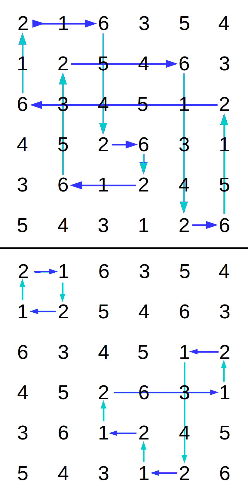
Figure 1 - Circuit paths in a Latin square
In a two-colored graph from a Latin Square, it is possible to trace along a row-colored edge from a cell holding one selected label to a cell holding the second selected label. This row transition arrives at different column location in that same row. From there, trace along a column-colored edge to a new row having a cell containing the first label. Continue in this manner, alternately seeking cells with the first selected label and then the second, in the process tracing a path along edges of alternating colors. This relationship, induced by the two symbols, is called a matching. Because there are only two transition colors, it is a two-color matching. Because the link colors alternate in a strict sequence along each path, it is a two-color rainbow matching. [2]
A two-color matching in a Latin Square is represented as a kind of graph in which the node weights are always 2. This satisfies sufficient conditions, dating back to the Carl Hierholzer proofs regarding solutions to Euler's classic "Bridges of Königsberg" problem [3], for existence of cyclic paths along the graph edges that connect the nodes in the matching. Because every node is weight 2, if the graph is connected, there is a single path that forms a loop visiting every row and every column. Figure 1 illustrates some paths that can be traced within a Latin square along two different symbol matchings. If the traced path reaches every row and every column, and then the graph representing the matching is connected. However, a path in another matching in the same Latin Square might return to the initial row-column location before all rows and columns have been visited. In this case, the two-color matching partitions the nodes into a set of isolated sub-graphs — i.e., not connected. Each of those sub-graphs is connected and forms its own closed cycle.
To simplify terminology, this paper calls the process of path-following along edges from node to node in a two-color matching tracing a circuit, analogous to tracing the flow of electricity through an electrical circuit. A loop identified by this tracing process is accordingly called a circuit, and a two-color matching can have one or more circuits. Define circuit length to be the number of distinct rows (or equivalently, the number of distinct columns) reached while tracing a circuit. If the length of the circuit equals N, the matching is connected, and the circuit is called a circuit of maximal length. Keep in mind that this terminology does not imply novelty.
In general, Latin Squares have certain invariant properties when subjected to operations known as autotopisms[11]. The operations relevant in the present context are permutations of rows and columns. The matchings within a Latin Square are invariant with respect to permutations of the columns -- after columns are permuted, the successor symbols for a circuit trace remain in the same rows as they were before. For similar reasons, the matchings within a Latin Square are invariant with respect to permutations of the rows. Thus, permuting rows and columns of a Latin Square does not affect the structure of matchings or the number of circuits within them.
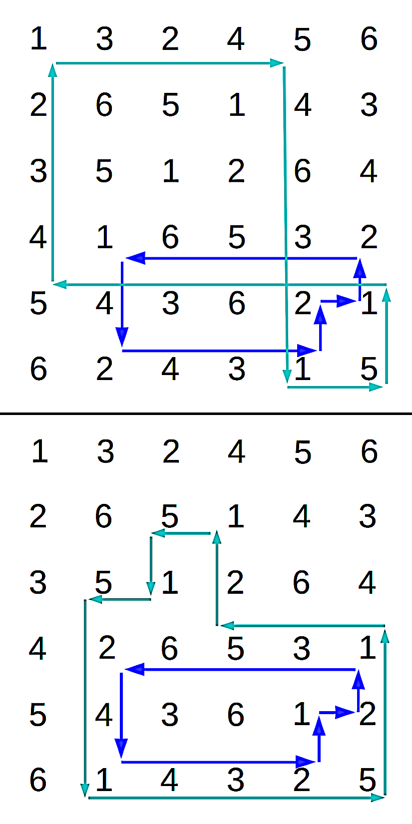
Figure 2 - Symbol swap in a 1-2 circuit
restructures a 1-5 circuit
Another kind of autotopism is a substitution mapping where an a new set of N symbols replaces the original set of symbols assigned to the cells. Clearly, such mappings are equivalent to selecting an alternative font for printing the contents of a given Latin Square; clearly, that would not have any effect on the internal structure. Swapping two symbols in only one circuit of a given matching preserves the Latin property, but it is not an autotopism — it can disrupt the structure of other matchings, as illustrated in Figure 2.
For a Latin Square selected at random from the set LS{N} of all possible Latin Squares of size NxN, each possible Latin Square is as likely as any other to be selected. Within these Latin Squares, the lengths of the circuits to be found within them can be described by a distribution. A pseudo-random Latin Square generator should attempt to deliver Latin Squares that exhibit the same probability distributions as truly random Latin Squares. Biases are differences between statistical properties of truly random Latin Squares and the Latin squares delivered by a pseudo-random generator method.
The "Latin square completion" problem has a long history. Colbourn [4] found that in general the complexity of the Latin square completion problem was NP-complete. Kuhl and Shroeder [5] show that even in the case of one empty row and one missing symbol, the completion problem remains nontrivial. A "divide and conquer" strategy proposed by DeSalvo [6] is also based on the idea of completion, partitioning the problem into an "easy" part and a "hard" part, where the scale of the "hard" part might be small enough to succumb to a brute force attack. However, this approach does not promise to scale up well for large Latin squares.
Given the challenges presented by a completion strategy, that idea is abandoned here. Unlike the classical "completion problem," prior symbol assignments are treated as advisory. Any prior symbol assignment is allowed to be altered in any manner that is expedient.
Phase 1 — Partial assignment with Latin constraints
We now begin the description of the new constructive algorithm, which we will call the Method of Circuits.
The new algorithm begins with a Latin Square layout for which every cell is empty. Empty cells are selected from the layout at random, without replacement. Each cell so selected is either assigned a symbol, or it is left empty, until each of the N2 locations has been processed one time.
Each label to be assigned to an empty location is subject to the Latin constraints. To determine which symbols can or cannot be assigned, each row is associated with a set of symbols that have not yet been assigned anywhere in that row. Similarly, each column is associated with a set of symbols that are still eligible to be assigned in that column. These symbol management sets are called "feasibility sets," where feasibility means that no Latin constraints are violated. Symbols eligible for assignment to an empty cell in the Latin Square layout are those symbols in the conjunction of the associated row and column feasibility sets. After a symbol is assigned to a cell at a given row-column location, that symbol is removed from the corresponding row feasibility set and also from the corresponding column feasibility set.
If it turns out that past label assignment decisions leave row and column feasibility sets that are disjoint, this situation is called a conflict. When such a conflicted cell is encountered, that cell remains empty, and the effort continues to find feasible assignments for the other empty cell locations in the layout, until the pool of unprocessed cells is exhausted.
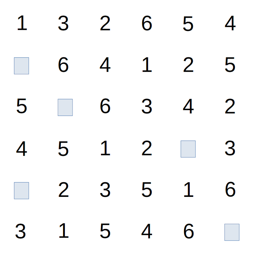
Figure 3 - Conflict cells remaining after
initial
filling phase
It is rare, but not impossible, that the symbol assignments randomly chosen in this manner result in completion of a Latin Square. In fact, any possible Latin Square could result this way, dependent entirely upon the results of the random selections. It is far more likely that there will be a number of cells that remain empty due to conflicts. Symbols that could not be successfully assigned remain in the row and column feasibility sets. Conflicted empty cells remain in the storage layout. Figure 3 illustrates a typical Latin Square layout after the initialization phase. Resolving the conflicts will occur in the next phase of the algorithm.
Phase 2 — Completion
Arbitrarily pick one of the empty conflict cells that remain after Phase 1 processing. We know that the column containing that cell has fewer than N assigned symbols. Similar for the column. However, the feasibility sets for row and column are disjoint, so no symbol can be assigned without violating Latin constraints.
Begin a circuit trace operation for a circuit within the partial Latin Square at the selected empty cell. Arbitrarily take one of the symbols from the set of feasible symbols available for assignment within the row of this cell. Call this the row symbol. Similarly, take one of the symbols from the set of feasible symbols available for assignment within the column of this cell. Call this the column symbol..
Artificially inject the row symbol into the empty cell. This causes no conflict in the row, but it can violate the Latin properties at one of the cells in the column. Locate the cell at which this occurs, and remove the row symbol from that location. We are now at an empty cell which is in the same column but at a different row than the cell that was last filled.
At the new empty cell, artificially inject the column symbol into the empty cell. This causes no conflict in the column, but it can violate the Latin properties at one of the cells in the new row. Locate the cell at which this occurs, and remove the column symbol from that location. We are now at an empty cell which is in the same row but at a different column than the cell which was last filled.
These actions alternate for filling an empty cell with a row symbol or a column symbol, and then clearing a conflicting symbol should it be present in that row or column. Each step reaches a row or a new column not previously visited. But recall that the layout is a partial Latin Square, and any row or column visited could have empty cells. If the symbol to be injected happens to be a symbol not previously present in that row or column, injecting that symbol does not produce a new conflict. The resolution process can then terminate.
We can observe that this process constitutes the trace of a partial circuit, augmented with an initializing assignment to get the trace process started, and a toggle operation that swaps row symbols and column symbols along the path — this is the same as the symbol swapping operation previously discussed in the Background and Prior Art section. Like any cycle trace operation, the path must either return to the cell at which the tracing started, or it must end because an empty cell prevents continuing further. In either case, the trace terminates in no more than 2*N steps.
Let us formalize the above process.
  RESOLUTION ALGORITHM FOR A CONFLICTED CELL

    Select one of the conflict cells.
    Make this conflict cell the current cell
    Repeat
      - let the new cell be the cell in the current column where the row
        symbol is already present
      - if NOT FOUND,
           inject the row symbol into the current empty cell
           TERMINATE resolution process.
      - if FOUND,
           clear the row symbol from the new cell
           inject the row symbol into the current empty cell
      - let the current cell be the new cell
      - let the new cell be the cell in the current row where the column
        symbol is already present
      - if NOT FOUND
           inject the column symbol into the current empty cell
           TERMINATE resolution process
      - if FOUND
           clear the column symbol from the new cell
           inject the column symbol into the current empty cell
      - let the current cell be the new cell
   End repeat
Theorem
Performing the conflict resolution process for every conflict cell present in the layout after Phase 1 results in a completed Latin Square.
Each circuit trace follows a circular path that must either arrive back at the cell where it started, to complete a circular cycle, or arrive at a row or column which is incomplete. In either case, the operation terminates with a path on which there is no symbol assignment conflict. Observe that each resolution sequence starts by injecting a symbol into the layout, and otherwise, symbols are either swapped or remain the same. That means, each circuit trace process leaves exactly one additional cell with an assigned label. Tracing a circuit, with or without toggling the symbols, preserves the Latin properties. Each trace sequence terminates in a finite number of steps. Because only a finite number of conflict cells exist before the resolution processing is applied, performing the conflict resolution operation at each conflict cell eventually completes the Latin Square construction in a bounded number of steps.
Complexity
The first phase of the algorithm performs exactly one operation at each of the cells in the layout. That operation either assigns a symbol to that cell, or assigns nothing to it. If there were never any conflicts, complexity of the construction algorithm is (trivially) O(N2). However, the occurrence of conflicts is more likely. For each cell, there is a process involving multiple cells to clear the conflict. Thus, the order must be higher than O(N2).
We know that the conflict resolution is based on circuit tracing. Each trace operation can visit at most 2*N cells (the case of a maximal circuit), which makes the trace operation no worse than O(N). The number of cells at which conflicts occur cannot exceed N2, the total number of cells in the layout. Thus, the combination of the Phase 1 and Phase 2 processes must have complexity higher than O(N2) but no higher than O(N3).
Empirical testing can observe that the number of conflict cells actually grows more slowly than the number of cells in the Latin Square layout, indicating a complexity less than O(N3). This behavior is illustrated in Figure 4.
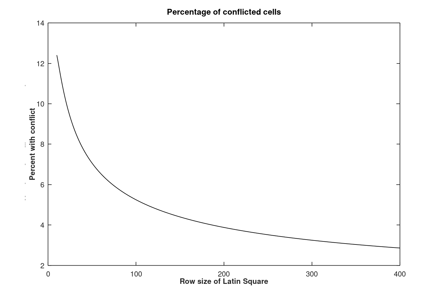
Figure 4 - Larger layouts experience a declining
rate of cell conflicts
To follow up on this observation, Figure 5 show the direct relationship between the number of conflict cells and the square size N. The curve would be linear if the number of conflicts was in proportion to the number of cells present. The superimposed regression curve is obtained using a least squares fit with weighting factors 1/N, using the conflict counts for square sizes up to 80x80; that regression curve is then projected to predict the number of conflicts for square sizes up to 400x400. It is found that a best-fit N1.56 growth rate parameter produced an excellent predictor for the number of conflict cells actually observed.
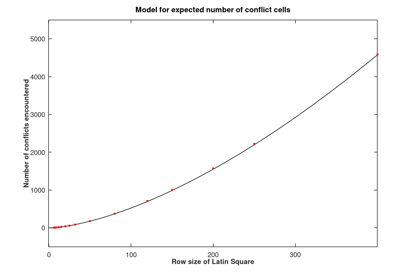
Figure 5 - Number of conflicts as a function of N
Further study would be needed to obtain a more accurate value of the growth rate parameter, but there would not be a lot of benefit from this. Better would be a theoretical explanation of how this particular dependency occurs.
If the assumption were correct that O(N) effort was required to perform each conflict resolution operation, the total effort to complete the Latin Square would be O(N2.56). Using visits to cells (equivalently, label assignments or reassignments) as a measure of effort, the following relationship was observed empirically by counting all label assignments made during the course of conflict resolution from a sampling population of 10 million generated Latin Squares. A weighted least squares best fit is again used to estimate the growth rate, producing the following relationship.
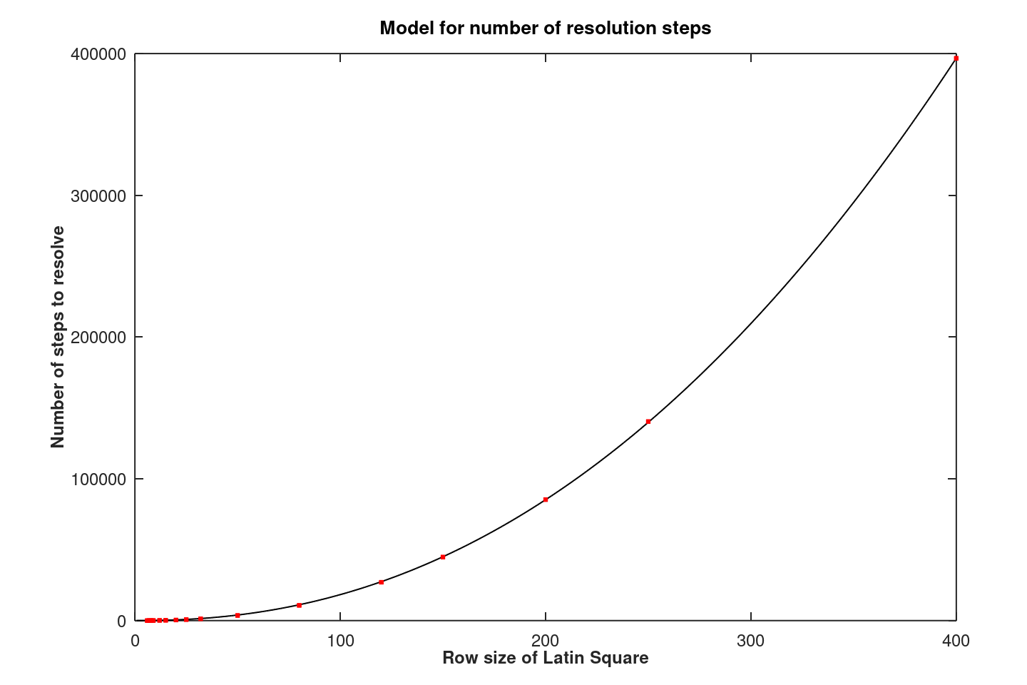
Figure 6 - Total effort for conflict resolution as a function of N
The observed growth of O(N2.22) rather than O(N2.56) indicates that effort expended for each conflict resolution is less than O(N). This should be no surprise, since each conflict resolution sequence can terminate early at rows or columns where empty conflict cells exist. As Figure 5 demonstrates, there are many more conflict cells than rows (or columns), so abbreviated traces occur much more often when Latin Squares are larger.
On the basis of this empirical evidence, using 9/4 as an approximation for the empirical estimate 2.22, a net complexity of about O(N9/4) is indicated.
A practical concern is computational efficiency, as opposed to order of complexity. Based on the data of Figure 6, a useful rule of thumb is that the total number of cell visits is bounded by 3 * N2, which includes the N2 operations required to supply the initial random assignments. For Latin Square sizes large than 150x150, higher-order effects start to dominate, and this rule of thumb no longer applies.
Bias
It is not easy to see how bias arises, but it demonstrably does.
Random Latin Squares have a property that a circuit selected at random from a matching generated by a pair of symbols selected at random will be maximal with probability P(N) = e/N, where e is the natural base of the logarithms.[7] By examining a large number of Latin Squares, and by counting the number of circuits with maximal length, it is possible to determine whether maximal-length circuits are over-represented or under-represented in a large population of Latin Squares that a generator algorithm produces.
The following TABLE 1 compares the probabilities for truly random Latin Squares and Latin Squares as delivered at the completion of Phase 2 of the Circuits algorithm. The reference probabilities are from a provided tabulation[7], and empirical estimates are obtained by sampling and testing populations of 10 million generated Latin Squares.
     TABLE 1 -  Probability of encountering circuits
         of maximal length in generated Latin Squares

size       reference        empirical test after
           (truly random)   Circuits algorithm Phase2

6x6         0.4286              0.4686
7x7         0.3876              0.4092
8x8         0.3399              0.3563
9x9         0.3021              0.3160
10x10       0.2717              0.2828
11x11       0.2472              0.2561
12x12       0.2266              0.2342
13x13       0.2091              0.2156
According to this criterion, it is apparent that the new algorithm, without any corrective measures, is subject to a small bias that consistently favors the presence of more maximal-length circuits than would be expected in truly random Latin Squares. A possible explanation is that a conflict resolution trace will tend to extend an existing circuit path, thus introducing a slight bias toward making circuits longer.
If we consider in more detail the size of the errors, and take into account that there are N*(N-1)/2 distinct symbol matchings possible in every Latin Square of size N, we can calculate how the bias relates to the expected number of maximal circuits for each Latin Square, as illustrated in TABLE 2.
   TABLE 2 - Expectation of the excess number of
      maximal circuits in generated Latin Squares, Phase 2

N         label pairs     excess           count of excess
           N * (N-1)/2    probabilities    maximal circuits

6x6         15             0.0400           0.60
7x7         21             0.0216           0.55
8x8         28             0.0164           0.46
9x9         36             0.0139           0.50
10x10       45             0.0110           0.49
11x11       55             0.0089           0.49
12x12       66             0.0076           0.50
13x13       78             0.0065           0.51
This looks like an expectation of approximately 1/2 more maximal-length circuits than truly random Latin Squares should have.
Phase 3 — Bias compensation
In an effort to find a corrective action that can counter the bias in maximal-length circuits, a new splay operation is introduced. The full details are presented in the appendix of this paper. In effect, a maximal circuit is split at two arbitrary locations. Then the two partials paths are forced to close, creating two circuits out of one. Doing this requires repositioning of some symbols, and these manipulations introduce new conflicts in some of the Latin Square cells. A circuit trace operation with label toggling is then applied to resolve the conflicts and restore the Latin properties, in much the same way that conflict resolution is done in Phase 2.
If one maximal circuit is removed from existence with each splay operation, we might naively expect that the count of maximal circuits should be reduced by 1, producing an expected shortage of 1/2 maximal circuit. However, this overlooks the side effects a splay operation has on other circuits, as was illustrated in Figure 2. It is not immediately clear what result to expect.
TABLE 3 shows the new levels of bias as observed from sample sets of 10 million Latin Squares, after one maximal circuit is identified in each Latin Square, and a splay operation is applied to that circuit. The new bias levels are compared to the previous results in TABLE 1.
   TABLE 3 - Excess probability of maximal circuits
      without and with an additional splay operation

N         bias in probability of         bias in probability of
          max-circuits, no adjustment    max-circuits, after splay

6x6          0.0400                        -0.0232
7x7          0.0216                        -0.0112
8x8          0.0164                        -0.0116
9x9          0.0139                        -0.0060
10x10        0.0111                        -0.0063
11x11        0.0089                        -0.0041
12x12        0.0076                        -0.0045
13x13        0.0066                        -0.0031
The sign is consistently inverted, and bias is consistently smaller, but not reduced by 1.0 maximal circuits as speculated.
Instead of applying a splay correction to every Latin Square produced, a rejection strategy is applied. A splay operation is applied only part of the time. The rest of the time, no adjustment is applied. The percentage of the cases receiving a splay correction is made to be an adjustable parameter, which is tuned empirically. Using a correction parameter value of 2/3 (a splay adjustment is applied 2/3 of the time) the results shown in TABLE 4 are obtained.
   TABLE 4 - Change in probability of maximal circuits after
      applying an additional splay operation 66% of the time

N         bias in probability of         bias in probability of
          max-circuits, no adjustment    max-circuits, after splay

7x7          0.0216                        -0.0002
8x8          0.0164                        -0.0022
9x9          0.0139                         0.0001
10x10        0.0111                         0.0005
11x11        0.0089                         0.0004
12x12        0.0076                        -0.0010
The remaining bias is at the limits that the empirical testing can distinguish from zero. However, we can say with certainty that bias in the number of maximal-length circuits is significantly reduced by the splay adjustments.
To put this into perspective, let's compare to the bias in the results generated by the popular Jorgenson-Matthews (J-M) algorithm [8], as obtained by similar testing. The comparison is shown in TABLE 5, where all entries are accurate to approximately 3 decimal digits.
     TABLE 5 -  Probability of encountering maximal cycles in
      Latin Squares generated by Jacobson-Matthews algorithm

size       reference       new algorithm after       J-M algorithm
           (truly random)    0.66 splay adjustment

7x7         0.3876          0.3874                    0.3962
8x8         0.3399          0.3377                    0.3438
9x9         0.3021          0.3022                    0.3050
10x10       0.2717          0.2722                    0.2737
11x11       0.2472          0.2476                    0.2488
12x12       0.2266          0.2256                    0.2272
The Jacobson-Matthews algorithm produces results with demonstrably more bias — though the levels are all very small. For Latin Squares of size 12x12 or larger, differences from true randomness are too small for the screening test to distinguish reliably. Practical applications might consider these levels of bias and their differences immaterial.
The splay operation depends on finding an arbitrary maximal circuit to split. O(N2) operations are required to find this circuit. Once that is done, one operation of O(N) will break and restructure that circuit. While these calculations add to the overhead, they do not increase algorithm complexity.
Instead of a comprehensive search, Monte Carlo random testing can be used. Limit the search for a maximal circuit to a maximum of 2·N tests of randomly-selected symbol pairs. There is less computational overhead than the complete search, but algorithm complexity is not affected. However, the truncated search will occasionally fail to find a maximal circuit, and a nominally "required" splay operation is missed.
The probability of failing to identify a maximal circuit in one random draw of a symbol pair from a random Latin Square is: F ≡ (1 - e/(N)). The probability of repeating this random testing 2*N times in sequence, and not finding a maximal circuit, is therefore F 2N. TABLE 6 shows some values for this to estimate how often the truncated testing is expected to fail to find any maximal circuit.
     TABLE 6 -  Probability of failing to detect a maximal
         cycles after 2*N attempts

  N          F           2N         F^(2N)
           (1 - e/(N))

   6       .48028        12         0.015 %
  10       .70595        20         0.095 %
  15       .80926        30         0.175 %
  20       .86145        40         0.257 %
  32       .91304        60         0.296 %
  64       .95703        128        0.361 %
   ...
  1024     .99734        2048       0.431 %
For all Latin Squares of practical size, the probability that a beneficial splay operation will be incorrectly omitted is under 0.005. Therefore, by this informal argument, it is recommended that if a suitable circuit of maximal length is not found within 2*N attempts, omit the Phase 3 splay operation.
Questions for Future Study
While the new Method of Circuits algorithm can provide immediate practical benefits, it leaves a number of unanswered questions.
The Phase 1 processing seems like a relatively straightforward sampling process, but in two dimensions. What probability distribution governs the number of conflict cells produced during this processing?
The effort required for Phase 2 processing depends on the effort required to trace partial circuits, which in turn depends on the distribution of circuit lengths. The only term of this distribution which has been characterized is the one for the maximal-length circuits.[7]
A theoretically rigorous complexity bound for the algorithm will depend on the answers from the previous two questions.
Is there an "optimal value" for the heuristic "splay parameter?"
To what extent does the splay operation correct for bias, and how much does it just displace bias from maximal length circuits to circuits of other lengths?
Does a splice, the reverse operation of a splay that merges two partitions of a matching, have any beneficial applications?
Are there other criteria that can expose different bias deficiencies in the new algorithm?
Conclusions
Several features of the new algorithm become apparent in a comparison to the popular Jorgenson-Matthews algorithm which, at the time of this writing, is the best-known practical method for producing pseudo-random Latin Squares of reasonable quality.
Chart 1 - Comparison of algorithms
| J-M Algorithm | Circuits Algorithm | |
| 1 | Requires a Latin Square as starting pattern | No starting pattern required |
| 2 | 2 N2 access operations for initial permutation | No initial permutation - construction is inherently random |
| 3 | Requires 3 N2 storage | Requires 5 N2 storage |
| 4 | Iterative, no established termination criterion, 3 N2 "moves" suggested | Terminates in finite steps |
| 5 | Requires 3 random variates for every "move" operation | Requires N2 random variates |
| 6 | Detectable maximal circuits bias in small squares | Negligible maximal circuits bias |
All of the points in Chart 1 require further comment.
-
The J-M algorithm is a "copier" followed by a "shuffler" rather than a direct "generator." N2 storage access operations are necessary to fetch a copy of an initial Latin Square pattern from storage, or to regenerate a well-known pattern algorithmically. The Circuits method generates an initial fill randomly, and does not require a starting pattern.
The correlation to the symbol locations in the start pattern used by the J-M algorithm must be broken. A simple random row-column permutation is effective, at the small cost of additional storage access operations. No permutation is needed for the Circuits algorithm.
The J-M algorithm is assumed to use only a 2-dimensional Latin Square structure for data storage. This is contrary to established literature stating that the J-M algorithm requires a third-dimension expansion into a sparse grid upon which the shuffling "moves" are applied, and then the final result is collapsed back to the original two dimensions. A separate paper[9] demonstrates, however, that the J-M algorithm implementation does not actually require any such expansion.
Both algorithms are assumed to maintain back-indexing arrays, so that a line search operation to locate a conflicting symbol within a row or column reduces to an O(1) array lookup. Thus, a significant part of the storage requirement, in both cases, is for the indexing arrays. As a practical matter, line searches can be substituted for the indexing arrays, reducing storage requirements by 2 N2 in both cases, with a corresponding efficiency and complexity trade-off.
The shuffling process of the J-M algorithm must continue until the statistics are "good enough." There is no firm rule about what this means. The 3 N2 "move" termination heuristic[9] suitable for "small" Latin Squares is assumed here, lacking anything more definitive; use your own judgment. In contrast, the Circuits algorithm is not iterative and requires no judgment call. It fills the layout cells systematically, and terminates.
Under the assumptions of item 4, the J-M iterations will typically use about 9 times as many random variates as the Circuits algorithm. Eventually, the higher-order character of the Circuits algorithm will catch up, but this doesn't occur until the size parameter N is large.
Reiterating empirical results presented previously: the J-M algorithm has a small but demonstrable bias in the number of maximal-length circuits in its smaller layouts. The Circuits method does not have this bias to any significant level. Either method might exhibit other forms of bias. For sizes larger than 12x12, the results of the two methods are almost indistinguishable from each other or from the theoretical ideal.
There should be no presumption that the Method of Circuits generates Latin Squares that are truly random. In particular, bias can manifest in different ways, and some means of testing should be able to detect these. However, applications that do not critically depend on true randomness are likely to find the deficiencies irrelevant, and can take advantage of the efficiency of the new algorithm now, while awaiting future theoretical studies.[10]
Appendix - Splay operation
This section provides details of the splay operation.
A splay operation is initiated at a randomly-selected cell such that it participates in a circuit of maximal length. Its label defines the first label that generates the circuit. The second label is the other label that implies the circuit of maximal length.
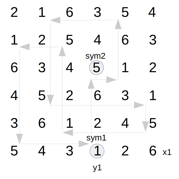
Figure 7A - Starting cell on
maximal circuit
- The "start cell" for the splay operation is the cell in the selected column containing the first label. Call this label sym1. Call this column y1.
- Let the row location of the starting symbol sym1 be called x1.
- In column y1, locate the second symbol, call this sym2, that in combination with sym1 implies the cycle of maximal length.
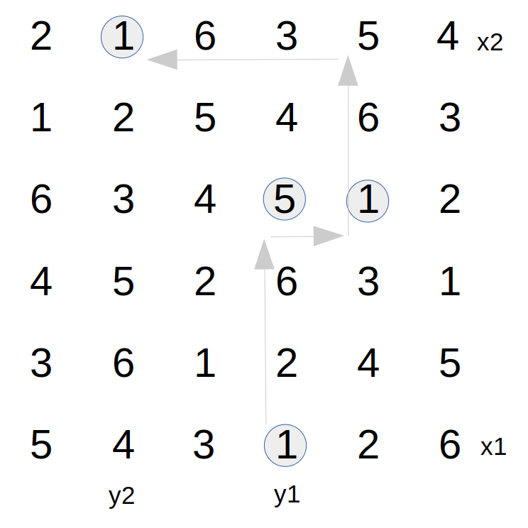
Figure 7B - Find locations of
circuit split
Trace along this circuit, advancing a randomly selected 1 to N-2 rows. This establishes a "split" location that does not return to the original row at the next step.
- Select any column other than y1, such that symbol sym2 is not in the same row as the starting location. Call this selected column y2. In column y2, let the row location of symbol sym1 be called x2.
Restructuring this circuit caused some label assignment conflicts. Identify cells where these conflicts occur.
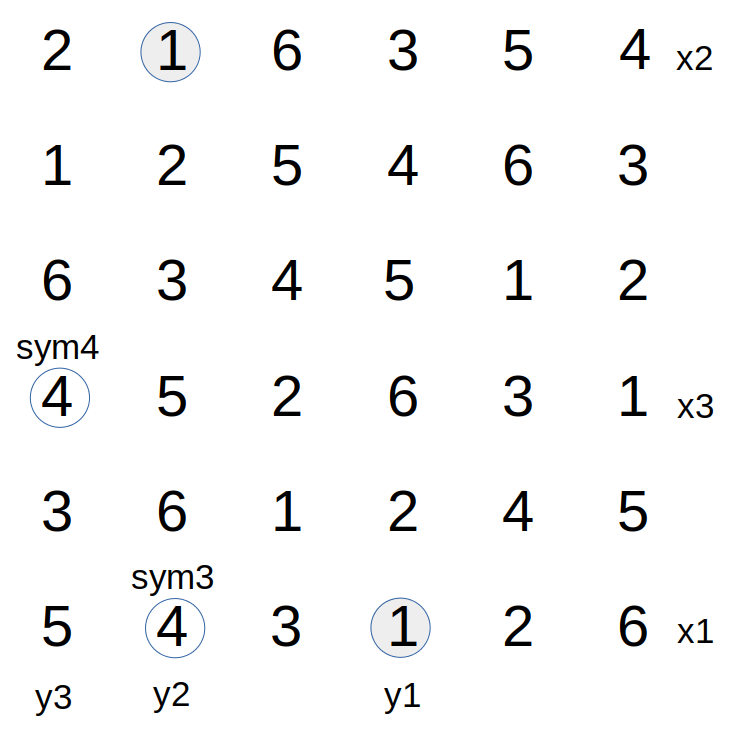
Figure 7C - Find cell locations of
label conflicts
- Find the symbol located at x1, y2. Call this symbol sym3.
- Find the row in column y2 where symbol sym2 is currently present. Call this row x3.
- Find the column within row x1 where sym2 is currently present. Call this column y3.
- Let the symbol currently present at location x3, y3 be called sym4.
Empty the cells that are going to be affected by conflict resolution.
- Clear the following cell locations:
-- location x1, y2 where sym3 was previously present
-- location x3, y2 where sym2 was previously present
-- location x3, y3 where sym4 was previously present
-- location x1, y3 where sym2 was previously present
If it happens that sym3 is the same symbol as sym4, perform the following actions to refill the empty cells and resolve the conflicts.
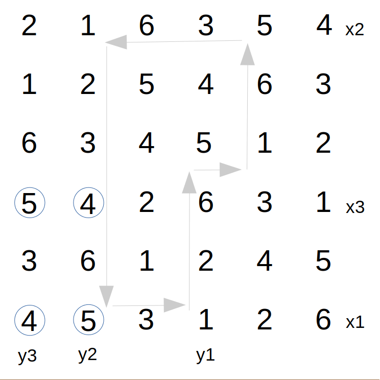
Figure 7D - Locate and refill cells
to resolve conflicts
- Inject symbols into the empty cells as follows:
-- sym2 is assigned to location x1, y2 where sym3==sym4 was previously present
-- sym2 is assigned to location x3, y3 where sym4==sym3 was previously present
-- sym3 is assigned to location x3, y2 where sym2 was previously present
-- sym3 is assigned to location x1, y3 where sym2 was previously present
These new label assignments restore the Latin property of the Latin Square layout and complete the splay operation.
For cases where sym3 and sym4 are different, instead perform the following actions.
- Inject symbols into empty cells as follows:
-- sym2 is assigned to location x1, y2 where sym3 was previously
-- sym2 is assigned to location x3, y3 where sym4 was previously
- Set some trace control variable values as follows:
-- xcur is set to x1
-- ycur is set to y3
- Find symbol sym4 in row xcur and call its column index ynext. If sym4 cannot be found in row xcur, insert symbol sym3 at location xcur, ycur. Then insert symbol sym3 at cell x3, y2 and skip to step 15. Otherwise, when sym4 is present in row xcur, clear the location xcur, ynext. Insert symbol sym4 at location xcur, ycur. Set ycur to ynext.
- Find symbol sym3 in column ycur and call its row index xnext. If sym3 cannot be found in column ycur, insert symbol sym3 at location xcur, ycur. Then insert symbol sym4 at cell x3, y2 and skip to step 15. Otherwise, when sym3 is present in column ycur, clear the location xnext, ycur. Assign symbol sym3 at location xcur, ycur. Set xcur to xnext, and jump back to step step 13.
- The splay operation is complete
At the completion of the splay process, observe the following net results:
- in row x1, the symbols sym2, sym3, and sym4 are in transposed positions, but all remain present in the row;
- in row x3, the symbols sym2 and sym4 are in transposed positions, but all remain present in the row;
- in all other rows, either the symbols sym3 and sym4 are in transposed positions or are unmoved;
- in column y2, the symbols sym2, sym3, and sym4 are in transposed positions, but all remain present in the column;
- in column y3, the symbols sym2 and sym4 are in transposed positions, but all remain present in the column;
- in all other columns, either the symbols sym3 and sym4 are in transposed positions or are unmoved.
No symbol that was present in any row or in any column has been removed from that row or column, so the Latin Property of the layout has been preserved.
The most important feature is that the assignment of the sym2 to the location at x1, y2 in step 10 or 11 results in the trace of the sym1, sym2 circuit to be rerouted to the starting row at the next step, where previously the trace would have continued on to visit other rows.
The effects on other circuits that involve either the first or second symbol are unpredictable. Possibly those circuits are split as well, but possibly they are spliced together to produce longer circuits.
References:
[1] Diestel, Reinhard, "Graph Theory"; 5th Edition (2016). Graduate Texts in Mathematics, Volume 173, Springer-Verlag; Heidelberg Graduate Texts in Mathematics, Volume 173.
[2] Gyárfás, András; Sárközy, Gábor N. "Rainbow matchings and cycle-free partial transversals of Latin squares"; Discrete Mathematics 327 (2014), 96–102.
[3] Hierholzer, Carl; Chr. Wiener (1873). "Ueber die Möglichkeit, einen Linienzug ohne Wiederholung und ohne Unterbrechung zu umfahren". Mathematische Annalen" (1873) Ch 6 pp. 30–32.
[4] Colbourn, C. J., "The complexity of completing partial Latin squares" Discrete Applied Mathematics 8(1) (1984), 25–30.
[5] Kuhl J, Schroeder M.W., "Completing partial Latin squares with one nonempty row, column, and symbol", The Electronic Journal of Combinatorics 23(2) (2016), #P2.23
[6] DeSalvo, Stephen, "Exact sampling algorithms for Latin squares and Sudoku matrices via probabilistic divide-and-conquer" (2016), arXiv:1502.00235.
[7] Trammell, Larry, "Screening Test for Latin Square Randomness using Matchings" (2023, unpublished), draft available at //www.ridgerat-tech.us/latinsq/bias/BiasTesting.html .
[8] Jacobson, M. T.; Matthews, P. "Generating uniformly distributed random Latin squares"; Journal of Combinatorial Designs 4 (6)" (1996), pp 405–437 .
[9] Trammell, Larry, "A Better Jacobson-Matthews Latin Square Shuffler" (2023, unpublished), draft available at //www.ridgerat-tech.us/latinsq/jmmethod/JMMethod.html .
[10] Trammell, Larry, implementations in Python distributed under the open source Creative Commons CC-BY License. For the basic version, rlatin5MOC.py.
[11] Stones, Douglas S; Vojtěchovský, Petr; Wanless, Ian M. "Cycle structure of autotopisms of quasigroups and Latin squares", Journal of Combinatorial Designs (2012), Vol 20, Issue 5, Pages 227-263.
This page and its contents are licensed under a Creative Commons Attribution 4.0 International License. For complete information about the terms of this license, see http://creativecommons.org/licenses/by/4.0/. The license allows copying, usage, and derivative works for individual or commercial purposes under few restrictions.
Document history:
Version 1.0 draft prepared in HTML format by Larry Trammell, copyright holder, who released the document irrevocably 2022-09-03 under the terms of the CC-BY-4.0 license.
Version 1.1 draft prepared in HTML format by Larry Trammell, who revised the document 2023-09-07 to link to example implementations and new cited documents, under the terms of the CC-BY-4.0 license