Background
The companion page discusses some presumably new ideas about using correlated rather than white noise generator stages for producing digitally-synthesized approximate pink noise, with a randomization strategy that eliminates the consistent spectral inaccuracies that the Voss-McCartney (V-M) algorithm produces. But the V-M algorithm still has some big advantages: it is very efficient, and it has very uniform processor loading for predictable timing in real-time applications, and the spectral anomalies, though large, appear to be localized and unbiased. For a description of that algorithm see the definitive site for pink noise generation, http://www.firstpr.com.au/dsp/pink-noise/.
With a randomized updating policy rather than a fixed one, it is not possible to know in advance which generator stages will update at any given time, so the computational loading at any given instant varies from nothing to the worst case that every generator stage is updated. The goal here is to apply the correlated generator approach but avoid the uneven loading and its drawbacks. If possible: improve accuracy and increase the spectrum coverage.
I will have to report only modest success in improving upon the numerical results obtained previously. There is some residual approximation error, and very little remaining freedom to try to improve upon it. I consider the design as shown in this page the end of the line for development of this approach — but of course, someday there could be departures that revitalize the idea.
For those who want to investigate further, I recommend starting from one of the contributed code submissions:
pinkgen.c An implementation example in C.
pinkclass.cpp
an implementation in C++.
avr_pinkgen.asm an example in an assembly language, using filter weights implemented with a hardware resistor network. More about this idea is available in an archived page from an earlier site.
A More Consistent Evaluator
Like the Voss-McCartney algorithm, this approach maintains a set of generator stages, updated at different rates. The difference is that the updating rate is only a statistical average, and is never performed on a predictable schedule (which is the source of the spectrum anomalies that plague the V-M results).
The new twist is this: the updating of the generator stages is made conditional, rather than independent. Stage 1 is updated only on the condition that Stage 2 through Stage N are not updated! Similar idea for the rest of the stages. This produces a different random process than when the stages are updated completely independently, but the generators retain the same probabilities of updating. By updating at most one stage at any given update opportunity, almost uniform processor loading is achieved.
There is a price for this. Whether one generator can update at any given time depends on what the other generators are doing, so there is no longer complete statistical independence. This lack of independence shows up as signals are combined. There is just enough difference to make the helpful theory about signal energy distributions unusable to guide the design. So I gave my best shot for normalizing the residual errors manually. The results shown here are not optimal, but close.
Let's Get To The Point, Shall We?
Okay, here is the algorithm that includes a coefficient set to cover approximately 9 octaves conforming to the "pink" 1/f power distribution. First, we need to define the parameters. The pP and the pA parameters are the amplitude scaling and probability of update parameters described in the previous note.
pA =   [  3.8024    2.9694    2.5970    3.0870    3.4006  ]
pP =   [  0.00198   0.01280   0.04900   0.17000   0.68200 ]
pSUM = [  0.00198   0.01478   0.06378   0.23378   0.91578 ]
The pSUM values are obtained by forming a running sum of the terms in the pP array. You should note that the values must sum to less than 1.0 for this algorithm to work.
You also need two other things. You need a pseudo-random number generator 'rand' that produces reasonably random values in the range 0.0 to 1.0, suitable for signal generation. You need an accumulator array 'contrib' that maintains the values currently contributed by each generator stage. You can initialize it randomly or fill with zeroes.
contrib = zeros(Nterms)
Now for each new time sample, perform the following update to determine the pink noise generator value.
   ur1 = rand;
   for stage=1:Nstages
      if (ur1 <= pSUM(stage))
         ur2 = rand;
         contrib(istage)=2*(ur2-0.5)*pA(istage);
         break for;
      endif
   endfor
   genout = sum(contrib);
We can observe that the update always uses one random value to determine which stages (if any) to update. There is a small probability that none of the stages are updated. An update operation uses a second random value. Auto-correlation results when values are not updated, with statistical properties discussed in the previous note. The number of random values required is 1 or 2, averaging a little less than 2, so the cost of evaluation is almost the same as the V-M algorithm.
Algorithm Variants
If you are using exact (fixed point) arithmetic, you can avoid summing the values of the generator stages to obtain the final output. Maintain the combined sum in another accumulator variable. To update, after a generator stage is selected, subtract the previous value of its contribution from the output accumulator, save the new contribution level, and add the new value into the accumulator. The generator output then equals the value of the accumulator variable.
The scaling shown is very arbitrary. The worst possible case for a fixed point implementation is when all of the random values reach 1.0 at the same time. With the scaling parameters shown, the generator would output its maximum level of 15.8564. Observing that 32767/15.8564 = 2066.48, you can scale all of the amplitude coefficients by 2066.48 to obtain a generator that does not exceed a signed 16-bit fixed point range.
You can balance the loading to a uniform 2 random evaluations per update by generating and discarding a value in the special case where none of the stages are updated.
If you have a 32-bit random number generator, you can apply some additional arithmetic to avoid one of the random number evaluations. A 32-bit generator might cost more than a 16-bit generator twice as shown. Otherwise, observe:
- If stage 1 is updated, we know the value of
ur1is in the interval 0.0000 to 0.00198. Values of a uniform distribution are uniformly distributed in a subset of the interval, so we can deriveur2 = ur1/pP(1)
- If stage 2 is updated, we know the value of
ur1is in the interval 0.00198 to 0.1280. Values of a uniform distribution are uniformly distributed in a subset of the interval, so we can deriveur2 = (ur1-pSUM(1))/pP(2) - Similar for stage 3,
urv = (uru-pSUM(2))/pP(3) - ... and so forth
You can get slightly faster execution by reversing the order of the stages. I present them from lowest frequency to highest, but the number of branches taken during evaluation is minimized using the reverse order. If you do this, be sure that the pSUM array is recalculated to match (don't just reverse the numbers)!
The previous note provided 3-stage, 4-stage and 5-stage generators. There is really no point in the 3-stage or 4-stage generators any more. If it turns out that there is too much low-frequency power, you can high-pass filter the noise sequence. You can drop one or two stages with the lowest probabilities of updating, and this will have a similar effect but you wont have much control over it.
Performance
Efficiency is close to as good as you can get of course. While there is no place in the spectrum where the signal energy is off to the degree that it is with the V-M algorithm, the anomalies there are highly localized, whereas here the anomalies in this algorithm are smaller and spread.
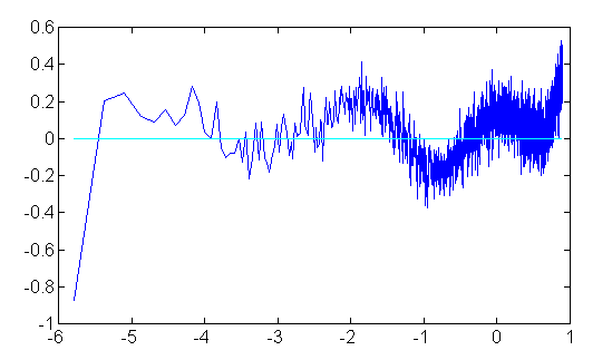
A plot of approximation errors is shown below. Using the parameter values given above for the generator, the x-axis range is in natural logarithms and corresponds to roughly the range 30 Hz to 18 kHz at 44kHz sampling, a little over 9 octaves. You can see the response droop near zero frequency, as expected because it is not possible to fit the singularity at frequency zero. You can also see where the levels starts to deviate from the 1/f model at the higher frequency end, approaching the Nyquist frequency. There is little power left at the very high frequencies so this shouldn't make any difference. The signal power should equal the 1/f model, hence the ratio should be 1.0. Computing the decibels for the ratio between actual response and the ratio curve, the plot should show a level line at 0.0 dB. As you can see, the deviations are about 0.25 dB, which corresponds to maximum amplitude deviation of about 2.9 percent. This should be close enough for all but the most demanding laboratory applications.
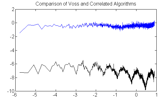
Just to give a little getter perspective on this, the new algorithm (5 generator terms) was run back-to-back against the Voss algorithm (12 generator terms). The Voss curve is artificially lowered so the two data sets don't overlap. Otherwise conditions are identical. The fuzz is uncertainty in the estimates, due to the limited sample size (just a few million points!) but the systematic variations are clearly visible. Draw your own conclusions.
Whether the new algorithm is the right one for you probably depends on how you intend to use it. It is easier to implement than the patterned scheduling of the V-M algorithm, with audibility good enough that you probably won't be able to distinguish it from a "true" pink process. If you need a laboratory grade noise source so you can depend on the correct energy distribution everywhere in the spectrum over the long term, this is not the best way to go.