Zone Circularity Algorithm

Abstract

Zone Circularity Defined

International standards such as IEC 1101 describe tolerancing specifications for manufactured machined elements, without providing any particular help in how to obtain or analyze measurements for evaluating the criteria. One such tolerance specification is "zoned circularity." This specification bounds a circumference between a largest inscribed circle and a smallest circumscribed circle, where the two circles have a common center. This center point is not necessarily the point that was intended as an axis point in the original piece design, and it is not necessarily a point of best balance because it is concerned with extrema of the deviations rather than the overall mass. To evaluate zone circularity from measurements, it is necessary to determine four parameters: two parameters identifying the radii of the bounding circles and two parameters locating the center point for these circles. Once these parameters are identified, the circularity zone estimate is the difference between the two radii.

Other Algorithms

An algorithm that I will call "the Simple Algorithm" is described by P. B. Dhanish in [1]. I will leave the discussion of prior state of the art to the introduction of that paper.

There is nothing specifically wrong with the Simple Algorithm. It is quite straightforward to implement. The problem is that real world data sets are not always in the right form to apply it. If a part is measured along three orthogonal axes with a general purpose CMM (coordinate measuring machine), the data set is in the appropriate form. However, this is not the way that high precision measurements are usually obtained. Usually a cylindrical piece is fixtured carefully on a rotation table, and radial deviations along a circumference are observed by a high precision linear displacement sensor. It is much easier to maintain tight tolerances using a one axis mechanism and a sensor calibrated over a very short range — but difficult enough even so.

Considering Step 17 of the Simple Algorithm in [1]: "Calculate the distance from the center of the circle to the translated coordinates." This calculation cannot be done using the radial deviation dataset alone because the absolute radial distance information is missing. The best that can be done is to supply a good estimate for average radius and "cook" the data by this amount. The algorithm is not at all sensitive to this adjustment, but nevertheless, the adjustment will introduce some higher-order error. This must be considered in the context of the algorithm described here, which has its own higher-order errors.

The survey of prior art in reference [1] also mentions a simplex search algorithm by T. S. R. Murthy [2], stating that it had the problem of no guarantees of optimality. This note also employs a simplex search, but the problem is formulated in such a manner such that the classic proofs of convergence for the Primal- Feasible Simplex Algorithm for Linear Programming (the LP problem, e.g. [3]) will assure convergence to the optimal solution in finite steps. In actual practice, the optimum is often achieved after four or five pivot operations.

Unmeasured Fixturing Error

When measuring a cylindrical part with a rotation table, great effort is put into fixturing the piece so that its center axis aligns with the rotation axis of the table. However, this is not perfect, so there are displacement errors, of roughly the same order as the tolerances that are being tested. In this section, we briefly discuss the impacts of centering on the measurement data set and obtain from this a motivation for the bounding functions used by the algorithm.

If measuring a perfectly circular, perfectly manufactured, perfectly centered part of radius R with perfect noise-free sensors, the sensors would see no radial change whatsoever, hence the data sets would be a "flat line." That is, displacement in radial direction is constant at every rotation angle.

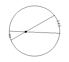
Now consider the impact of displacing the ideal object of radius R by a very small vector displacement r. We are not concerned about the direction of this displacement here, so for purposes of discussion consider this displacement to be in the direction of the x axis normal to the axis of rotation.

	It is apparent in this illustration (with size of center shift exaggerated to magnify the effects) that angles of rotation with respect to the table — which is all we can really control — no longer correspond to equal angles with respect to the part itself.
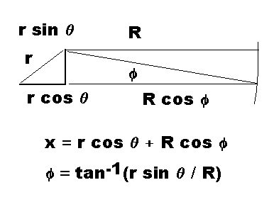
Analyzing the displacements with the assistance of the following vector diagram, we can observe that an expression for apparent radius, as measured at the circumference, is R' = r cos θ + R ( cos tan-1 ([ r sin θ]/R) )

where the terms are

When r is very much smaller than R, the complicated multiplier on term R is not significantly different from 1.0. In other words, a small fixturing displacement has the apparent effect of introducing a sinusoidal displacement of magnitude r through the data set. This wave will influence each measurement when measuring a less-than-ideal piece in less-than-perfect fixturing with real-world sensors.

With the displacements approximately sinusoidal, the apparent radial displacements will range roughly from R-r to R+r. It is possible to take the ratio of outside to inside radius (R+r)/(R-r) into account by providing reasonable prior estimates for R and r. However, the ratio is so close to 1.0 in practice that the effect is immaterial. Assume that the inner and outer bounding sinusoids have the same magnitude, accepting that this leads to an insignificant second order error in the bound estimates.

Formulation Of Problem

We know that the displacements introduced by any shift of the center, not just displacements due to fixturing errors, will have the same first-order effects discussed in the previous section. We know that the displacement effects upon measurement data are very nearly sinusoidal, hence they can be represented as a scaled sum of cosine and sine wave terms. We have assumed that the magnitude is the same for both boundary curves, so the model for these curves is:

 U(θ) = ru  +  ds sin(θ) + dc cos(θ)

 L(θ) = rl  +  ds sin(θ) + dc cos(θ)

where the terms in this expression are

The problem is to select values of variables ru, rl, ds and dc to minimize separation distance z = ru−rl, subject to the bounding conditions on the measured data set M

 M(θ) ≤ U(θ)
 M(θ) ≥ L(θ)

Bounding curves are defined as feasible if the constraints are satisfied, that is, if no data value is higher than the upper bounding curve U and no data value is lower than the lower bounding curve L. We can define feasible bounding curves in terms of slack variables. Define two non-negative slack variables for each measured term. Designate the slack variables for the upper bounding curve as row vector Su, and the slack variables for the lower bounding curve as row vector Sl. For the upper bound curve, the curve term minus a slack variable from Su yields the measured M value. For the lower bound curve, the curve term plus a slack variable from Sl yields the measured M value. If none of the slack variables are negative, this indicates that the upper bound is truly above all of the measurement terms and the lower bound is truly below.

While the sine and cosine curves are inherently nonlinear, these functions never change and can be pre-evaluated term by term, to yield constant vectors C and S respectively. Subsequently, the boundary curves can be considered a linear form, with variable multipliers applied to constant vectors. The combination of the linear constraints with the linear objective criterion and sign constraints on slack variables yields a classical linear programming problem.

To represent the problem in LP tableau form, let

• N be the number of terms in the data set,
• I1 be a constant vector of length N with all 1 terms
• I0 be a constant vector of length N with all 0 terms
• R0 be a constant row of length N with all 0 terms
• I be an NxN square unit matrix.

  rh  rl   ds  dc    Su    Sl
  ========================================
  I1  I0   S   C     -I    0     |   M
  I0  I1   S   C     0     I     |   M
  -------------------------------|--------
  1   -1   0   0     R0    R0    |  -z

All we need to do at this point is apply a classic linear programming solver with unconstrained sign on the first four variables and nonnegative sign restrictions on the 2N slack variables.

A well known result from the theory of linear optimization (see [3] or [4] for example) is that if an optimal solution exists (as it will for any adequate data set), a basic optimal solution will exist. As the four critical variables rh, rl, ds and dc will always be involved in the basic solution, this means that there will be four slack variables that are zero in the basic optimal solution. Hence, there will be four and possibly a few more "points of contact" between the two bounding curves and measured positions at the optimum.

Establishing An Initial Feasible Solution

While general simplex method solvers do not assume anything about the structure of the constraints, this particular problem has an extremely sparse special structure. The first N constraints can be scaled by -1 "on both sides" by inverting all signs in the first N rows. This results in the following equivalent tableau.

  rh   rl   ds  dc   Su   Sl
  =======================================
  -I1  I0  -S  -C    I    0     |  -M
  I0   I1   S   C    0    I     |   M
  ------------------------------|--------
  1    -1   0   0    R0   R0    |  -z

By inspection, the slack variable columns form a trivial basis, but not a feasible basis because positive slack variables cannot be equal both to a non-trivial measurement vector and to its negative. However, it is easy to construct an initial feasible basis by establishing flat- line bounding curves that contain the entire data set. Find the index kmax in the first N rows of the last column such that -M is minimum at kmax (i.e. M is maximum). Also find the index kmin in the second N rows such that M is minimum at row kmin.

For readers unfamiliar with conventional terminology of the LP problem, we digress briefly and define a pivot operation as a special set of row operations applied to a matrix. One nonzero term of the matrix is designated as the pivot element. For every matrix row k other than the row kp containing the pivot element, compute the ratio of the two terms in pivot column v: -v(k)/v(kp). Matrix row kp is then multiplied times this ratio and added to matrix row k. Finally, all of the terms in the pivot row are scaled by 1/v(kp). The net effect of the pivot operation is to zero all terms in pivot column v except for term v(k), which gets a value 1.0. Various other terms throughout the matrix are modified by the row operations in the process. Notice that the pivot affects the last cost row as well as the constraint rows, but there is no effect on identity matrix columns for which the nonzero term does not lie in the pivot row. Hence, we can omit these slack variable columns from the tableau, generating them easily when needed later.

To start, the first pivot operation is performed in the first column at location kmax, and in the second column at location kmin. These two pivot operations will have the effect of eliminating the nonzero cost coefficients from the last row under columns 1 and 2, creating new nonzero cost coefficients below columns 3, 4, 4+kmax and 4+N+kmin. One nonzero term remains in column one and in column two after the two pivot operation. The values in the last column in rows kmin and kmax provide initial bounds on the locations of the outer and inner bounding wave. The other terms of the modified last column will show the values of slack variables, which at this point are all positive. Columns 1, 2, and the slack variable columns except 4+kmax and 4+N+kmin form a feasible basic solution, though probably not optimal.

Introducing Sinusoids Into the Basis

We know that in the optimal solution we are seeking, there will probably be some adjustment to the center location for the bounding curves. The center point shift will result in a nonzero sinusoidal component. In anticipation of this, introduce variable ds and dc into the basis immediately.

The values of ds and dc are not sign constrained, so we need to modify the usual minimum ratio rule of linear programming for selecting a pivot element. Start with the third column, the one for variable ds. To locate the pivot element in this column, compute the following:

• Ignore any term that is in rows kmin, that is in row kmax, or that has a zero value.
• Ignore any term that has the same sign as the cost term at the bottom of the pivot column.
• For the remaining rows, compute the ratio of the last column term to the term in column 3.

Perform the same steps again, this time using column 4 as the pivot column instead of column 3, and also excluding the previous pivot row from the ratio test.

After completing these operations, there will be a single term with value 1 in each of the first four columns, and all other terms in these columns including the cost row will be 0. The pivot operations will result in changes to the values in the last M column, and will produce non-zero cost coefficient values at the bottom of as many as four slack variable columns. From this point on, the first four columns will remain in the basis and will not change; they can be ignored, and their pivot rows are not involved in subsequent ratio testing.

Improving the Basic Solution and Optimality

This section is just a brief review of the simplex solution method for the LP problem. Readers familiar with the algorithm can skip to the next section.

If all of the coefficients are zero or positive in the cost coefficient row, the current solution is optimal — any change to the basis must either make the optimality criterion worse or violate one of the sign constraints on a slack variable. Since the basis is full rank, the solution corresponding to that basis must be unique. Actually, it is rather common for a few extreme points to dominate the data set, hence it is not uncommon for the initial basis that includes the first four columns to be optimal.

At this point, if any of the four nonbasic slack variable columns has a negative cost coefficient, select that column as a new basis column. If there is more than one, the tie can be broken in any desired manner. This particular problem is not subject to the phenomenon of basis cycling so picking the column with the most negative cost coefficient is most likely to yield an optimal solution quickly.

For the elements in the selected pivot column, excluding the rows corresponding to the four permanent basis variables, find the pivot row kp such that in this row the term is positive, and the ratio of the term in the M column divided by the term in the pivot column is minimum. Pivot on the selected element.

Repeat all of the steps in this section until the condition for optimality is reached. For the same reason that it is not unusual to land upon an optimal solution immediately when first establishing the feasible basis, it is not unusual for a very small number of pivot operations to yield the optimum.

Once the optimum is reached, slack variables corresponding to columns that are not in the basis set are assigned the value zero. Nonzero slack corresponds to "points of contact" between the bounding curves and the measurement set. The terms of the last column in the rows having nonzero variables in columns 1 through 4 yield the parameter values for the bounding curves at the optimum. The estimate of the zone circularity is then obtained from subtracting ru - rl at the optimal solution.

Simplifying Computations

The 2N x 2N terms for the slack variables start as an identity matrix, and most of these terms never change. The columns that are actually needed can be generated on the fly. The following algorithm can be compared to the previous description to verify that it performs all of the same computations as the classical algorithm, yielding exactly the same solution, but generating data only when needed.

Establishing Initial Feasible Solution

1. Build a matrix with 2N+1 rows and 6 columns, initially all zeros.
2. Place the terms -M and M into column 1 with cost term 0.
3. Generate in column 2 a vector with all values 0 except for a term 1.0 in row kmax.
4. Generate in column 3 a vector with all values 0 except for a term 1.0 in row kmin.
5. Fill column 4 with one negative sine cycle, one ordinary sine cycle, and cost coefficient 0.
6. Fill column 5 with one negative cosine cycle, one ordinary cosine cycle, and cost coefficient 0.
7. Generate in column 6 a vector with all values -1 in the first N terms and all values 0 in the second N terms, plus one more cost term of 1.
8. Identify term kmax from column 1.
9. Pivot on term kmax in column 6.
10. Add kmax to the list of solution variable rows, associated with parameter variable rh.
11. Generate in column 6 a vector with all values 1 in the second N terms and all values 0 in the first N terms, plus one more cost term of -1.
12. Identify term kmin from column 1.
13. Pivot on term kmin in column 6.
14. Add index kmin to the list of solution variable rows, associated with parameter variable rl.

Introducing Center Displacement Variables to Basis

1. Copy column 4 to column 6.
2. Using column 6 and column 1, perform a test for pivot without sign restriction to find pivot row kp.
3. Zero all terms of column 4 except term in pivot row, which is set to 1.0.
4. Pivot in column 6 at the selected pivot row.
5. Add the pivot row index to the list of solution variable rows, associated with parameter variable ds.
6. Copy column 5 to column 6.
7. Using column 6 and column 1, perform a test for pivot without sign restriction to find pivot row kp.
8. Zero all terms of column 5 except term in pivot row, which is set to 1.0.
9. Pivot in column 6 at the selected pivot row.
10. Add the pivot row index to the list of solution variable rows, associated with parameter variable dc.

Locating the Optimum

Repeat all of the steps in this section until the initial test for optimality is satisfied.

1. Check the cost coefficients in the last terms of vectors 2 through 5. If they are all non-negative, the solution is optimal.
2. Select one of the non-basic vectors having a negative cost coefficient, usually the most negative one.
3. Copy the selected column to column 6.
4. Perform the ratio test to select a pivot element kp under sign restrictions, using column 6 and column 1.
5. Clear all of the terms in the original selected column except for the pivot row, which has a value 1.0.
6. Pivot in column 6 at the selected pivot row kp.

When optimality is reached, the index terms associated with columns 2 and 3 locate the terms in the first column where the values rh and rl can be obtained. For purposes of a simple tolerance evaluation, report the value rh-rl. The negative of this value will also appear as the last element in the first column of the optimal solution. For purposes of a more detailed presentation of the data, index terms associated with columns 4 and 5 locate the values of the ds and dc parameters in the first column. For all other row indices that are not associated with one of the solution variables, the first column provides the values of the slack variables at the optimum fit.

A Final Observation

The method described here for zoned circularity can be modified to solve the related problems of finding the minimal circumscribing circle and maximal inscribed circle. Having only one bounding curve, one of the radius parameters is omitted, one set of slack variables is dropped, and one group of N bounding constraints is dropped. This reduces the problem from a 2N+5 x 2N+1 system to a N+4 x N+1 system. Only three operations are required to establish the initial feasible basic solution, and there will be three or more "points of contact" at the optimum. In other respects, the method of solution is similar.

Appendix 1 - Simplified Numerical Example

The following data set contains six points of radial displacement measurement, at equal rotation angles, covering one object rotation.

   .0545; .0542; .0488; .0506; .0519; .0469;

After initial construction of the solution matrix first column, it is observed that the lowest number in the upper half of column 1 occurs in row 1, and the lowest number in the second half occurs in row 12. The basic slack variable columns with terms 1.0 in these two rows are constructed in columns 2 and 3. One negative cycle and one positive sine cycle appear in column 4. One negative and one positive cosine cycle appear in column 5. Column 6 is a working scratchpad column and is not shown.

 -5.4500e-002  1.0000e+000            0            0 -1.0000e+000
 -5.4200e-002            0            0 -8.6603e-001 -5.0000e-001
 -4.8800e-002            0            0 -8.6603e-001  5.0000e-001
 -5.0600e-002            0            0            0  1.0000e+000
 -5.1900e-002            0            0  8.6603e-001  5.0000e-001
 -4.6900e-002            0            0  8.6603e-001 -5.0000e-001
  5.4500e-002            0            0            0  1.0000e+000
  5.4200e-002            0            0  8.6603e-001  5.0000e-001
  4.8800e-002            0            0  8.6603e-001 -5.0000e-001
  5.0600e-002            0            0            0 -1.0000e+000
  5.1900e-002            0            0 -8.6603e-001 -5.0000e-001
  4.6900e-002            0  1.0000e+000 -8.6603e-001  5.0000e-001
            0            0            0            0            0

  5.4500e-002 -1.0000e+000            0            0  1.0000e+000
  3.0000e-004 -1.0000e+000            0 -8.6603e-001  5.0000e-001
  5.7000e-003 -1.0000e+000            0 -8.6603e-001  1.5000e+000
  3.9000e-003 -1.0000e+000            0            0  2.0000e+000
  2.6000e-003 -1.0000e+000            0  8.6603e-001  1.5000e+000
  7.6000e-003 -1.0000e+000            0  8.6603e-001  5.0000e-001
  7.6000e-003            0 -1.0000e+000  8.6603e-001  5.0000e-001
  7.3000e-003            0 -1.0000e+000  1.7321e+000            0
  1.9000e-003            0 -1.0000e+000  1.7321e+000 -1.0000e+000
  3.7000e-003            0 -1.0000e+000  8.6603e-001 -1.5000e+000
  5.0000e-003            0 -1.0000e+000            0 -1.0000e+000
  4.6900e-002            0  1.0000e+000 -8.6603e-001  5.0000e-001
 -7.6000e-003  1.0000e+000  1.0000e+000 -8.6603e-001 -5.0000e-001

When processing the nonbasic column 4, it has terms of sign opposite the cost coefficient (excluding rows 1 and 12) in six locations, with minimum ratio in row 9. After the column copy, and construction of nonbasic slack variable column with a 1.0 term in row 9, the pivoting operation yields the following.

  5.4500e-002 -1.0000e+000            0            0  1.0000e+000
  1.2500e-003 -1.0000e+000 -5.0000e-001  5.0000e-001            0
  6.6500e-003 -1.0000e+000 -5.0000e-001  5.0000e-001  1.0000e+000
  3.9000e-003 -1.0000e+000            0            0  2.0000e+000
  1.6500e-003 -1.0000e+000  5.0000e-001 -5.0000e-001  2.0000e+000
  6.6500e-003 -1.0000e+000  5.0000e-001 -5.0000e-001  1.0000e+000
  6.6500e-003            0 -5.0000e-001 -5.0000e-001  1.0000e+000
  5.4000e-003            0            0 -1.0000e+000  1.0000e+000
  1.0970e-003            0 -5.7735e-001  5.7735e-001 -5.7735e-001
  2.7500e-003            0 -5.0000e-001 -5.0000e-001 -1.0000e+000
  5.0000e-003            0 -1.0000e+000            0 -1.0000e+000
  4.7850e-002            0  5.0000e-001  5.0000e-001            0
 -6.6500e-003  1.0000e+000  5.0000e-001  5.0000e-001 -1.0000e+000

When processing the nonbasic column 5, it has terms of sign opposite the cost coefficient (excluding rows 1, 12 and 9) in six locations, with minimum ratio in row 4. After the column copy, and construction of nonbasic slack variable column with a 1.0 term in row 4, the pivoting operation yields the following. After the last two pivot operations, the ds parameter is associated with row 9 and the dc parameter is associated with row 4.

  5.2550e-002 -5.0000e-001            0            0 -5.0000e-001
  1.2500e-003 -1.0000e+000 -5.0000e-001  5.0000e-001            0
  4.7000e-003 -5.0000e-001 -5.0000e-001  5.0000e-001 -5.0000e-001
  1.9500e-003 -5.0000e-001            0            0  5.0000e-001
 -2.2500e-003            0  5.0000e-001 -5.0000e-001 -1.0000e+000
  4.7000e-003 -5.0000e-001  5.0000e-001 -5.0000e-001 -5.0000e-001
  4.7000e-003  5.0000e-001 -5.0000e-001 -5.0000e-001 -5.0000e-001
  3.4500e-003  5.0000e-001            0 -1.0000e+000 -5.0000e-001
  2.2228e-003 -2.8868e-001 -5.7735e-001  5.7735e-001  2.8868e-001
  4.7000e-003 -5.0000e-001 -5.0000e-001 -5.0000e-001  5.0000e-001
  6.9500e-003 -5.0000e-001 -1.0000e+000            0  5.0000e-001
  4.7850e-002            0  5.0000e-001  5.0000e-001            0
 -4.7000e-003  5.0000e-001  5.0000e-001  5.0000e-001  5.0000e-001

Inspecting the cost coefficients in the last terms of the four nonbasic columns 2 through 5, it is observed that all of these terms are positive, hence any pivot operation that re-introduced these slack variables into the basis would only serve to increase the separation of the bounding curves, contrary to the goal of minimizing the separation. Hence, an optimal solution is indicated. The optimal values of the ds and dc are picked from rows 9 and 4 in column 1. The radial separation between the two curves is picked from rows 1 and 12 of column 1. The difference is 4.700e-3, which is the width of the circularity zone. Alternatively, it can be observed that the negative of this result appears in the last term of column 1 and can be read out directly.

Footnotes:

[1] A simple algorithm for evaluation of minimum zone circularity error from coordinate data, P. B. Dhanish, International Journal of Machine Tools & Manufacture 42 (2002) 1589-1594.

[2] A comparison of different algorithms for circularity evaluation, T. S. R. Murthy, Precision Engineering 8-1 (1986) 19-23.

[3] A classic reference, Linear Programming and Extensions, G. B. Dantzig, Princeton University Press, 1963.

[4] A more recent text, Linear Programs and Related Problems , E.D. Nering and A.W.Tucker, Academic Press, 1990.