The Total Least Squares Problem

There is something that many people using Least Squares methods either don't know or choose to disregard. A Linear Least Squares formulation using Normal Equations and matrix methods assumes that the independent data are accurate, while uncorrelated noise affects the dependent data only.

That isn't necessarily a bad assumption. Often the "inputs" are signals that are controlled accurately, such as time^[1] observed to extreme precision by a digital clock, or position controlled by a high-gain servo loop. But suppose the input signal is "acceleration," as measured using a strain-sensing accelerometer? Or a thermocouple temperature measurement, where quantum noise levels are roughly the same magnitude as the Seebeck effect potentials? Maybe worse, what happens when there is strong correlation between the noise in the various input and output variables? In such situations, per strict theory, Least Squares shouldn't work so well. In practice, it will probably work well enough, but if you aren't sure, there are alternatives.

This section covers two techniques, an alternative method of analysis, and an idea of temporarily using supplementary outputs that are impractical, for various reasons, to observe during general operation.

 

Background tale: woe and confusion

Back in the good ol' days, I was working on a robotics trajectory problem. I wanted a model that predicted where a motion trajectory was pointing, based on a history of image sensor information. The flat 2-D image has two orthogonal axes, which depend on the manipulator structure to determine alignment in the real world.

There was a lot of mechanical momentum, so over any very short time interval, the motion acted very much like a linear system. So it made sense that "the x-axis position" and "the y-axis position" would have what looked line a kind of linear relationship. (This isn't a completely realistic view. Actually, the x-axis position and the y-axis position are similar functions of time, but not functionally dependent on each other.) Movements along the two axes were subject to similar kinds of small physical disturbances from vibrations, control dynamics, and so forth, and there was a small variance in position sensor estimates.

With a linear relationship, the y values could be considered linearly dependent on the corresponding x values. Or the x values could be considered linearly dependent on y values, and invert algebraically. Take your pick, the results should be the same, whichever seems most useful.

Except that this didn't happen. The "best fit" lines for y as a function of x were different from the "best fit" lines for x as a function of y, consistently. Differences were not very big, but they were very real, and very annoying. How is that possible? How can the same data, given the same weighting factors, produce two different "least squares best fits" for the same line?

It turns out that I should have been using a different fitting approach, one that finds a best linear relationship between x and y when both data sequences are noisy and neither one is necessarily a direct linear function of the other.

 

Introducing the Total Least Squares problem

Suppose that there is a strong linear relationship between the input variables m and predicted output variable y, and that we know the multiplier parameters p for this model. For a good model, we should have

    Σ( m * p ) ≈ y

for any set of corresponding inputs and output at any instant of time.

Consider then the expression

    Σ( m * p ) - y

If the model is really good, this number is very small, with no effects other than random noise remaining. The smaller it is, the better the model must be. This is the basic idea of a Total Least Squares^[2] analysis.

 

Preparing for the Total Least Squares analysis

There are some preconditions for a successful analysis.

1. You must have a reasonably good estimate of the model order. Results can be poor, and there can be numerical trouble, if your proposed model tries to fit parameters for too many or too few model parameters.

2. You must use input and output data values that are reasonably well scaled. This is important for Linear Least Squares, but perhaps more for Total Least Squares.

3. You must have a sufficient data set so that the input-output behaviors of the model are statistically distinguishable from the variance effects produced by sampling the random noise.

4. You should select variables that exhibit a high degree of independence. For example, if observing vibrations of an automobile body, it is probably a bad idea to include measurements of both the frame and hood, because the two are rigidly connected.

Suppose that the model data sets are obtained by driving your system with a randomized signal that spans the expected operating range in a balanced and uniform manner. At each instant, capture input and output variable values. Scale the data appropriately so that magnitudes are comparable. Record the input and output data as columns in a large matrix.

 

Example: system with two supplementary outputs

Suppose that the goal of the system modeling is a dynamic state transition model to predict one of the system outputs. However, with some extra instrumentation, it is possible on a temporary basis to observe two additional outputs. All of the values can have a certain amount of random noise. The test input signals are randomized, and uniformly span the input range, allowing the output levels to span their output range. The signal data are scaled and corrected for any constant offset, so that the model can be strictly linear.

Sets of the adjusted input and output values, as seen over time, are collected as history records.

• The x values are the input measurements. For this example, five past input values are used.
• The y values are the output measurements. For this example, only one recorded past output is used for each of the three output variables observed.
• The superscripts indicate the time (position in the dataset) where these samples appear — the more negative, the further into the past.

This model implies that, at each step, all outputs of the system start from what they were previously, and the input history sequence indicates how these output values change. Is that enough? We can try it and find out. Here is the organization for one history record collected during the testing.

$$\left[\begin{array}{ccccccc}{y_1}^{\left(0\right)}& {y_2}^{\left(0\right)}& {y_3}^{\left(0\right)}& x^{\left(0\right)}& x^{\left(-1\right)}& \dots & x^{\left(-4\right)}\end{array}\right]$$

Next, we need to include the predicted output values for the model. For the case of a dynamic state transition matrix, the desired dependent variable is the next predicted value for one of the output sequences. As with Linear Least Squares, the desired prediction sequence is a time shifted version of the output signal.

Somewhat arbitrarily, let's choose the first signal y1 as the one to be predicted by the model. Looking at the recorded data in the data set, add this "one time step in the future" output value as a new element at the front of each history record, producing an augmented history record. The augmented history records look as follows.

$$h^T\iff \left[\begin{array}{cccccccc}{y_1}^{\left(1\right)}\parallel & {y_1}^{\left(0\right)}& {y_2}^{\left(0\right)}& {y_3}^{\left(0\right)}& x^{\left(0\right)}& x^{\left(-1\right)}& \dots & x^{\left(-4\right)}\end{array}\right]$$

This is repeated for all of the recorded time steps in the data set. All of the augmented history records like this are organized as a matrix, M. Except for the inclusion of both input and output data in the columns, this matrix structure would otherwise be the same as the constraint data matrix for a typical Linear Least Squares problem.

$$M\iff \left[\begin{array}{cccccccc}{y_1}^{\left(1\right)}& {y_1}^{\left(0\right)}& {y_2}^{\left(0\right)}& {y_3}^{\left(0\right)}& x^{\left(0\right)}& x^{\left(-1\right)}& \dots & x^{\left(-4\right)}\\ {y_1}^{\left(0\right)}& {y_1}^{\left(-1\right)}& {y_2}^{\left(-1\right)}& {y_3}^{\left(-1\right)}& x^{\left(-1\right)}& x^{\left(-2\right)}& \dots & x^{\left(-5\right)}\\ \text{etc.}\end{array}\right]$$

For setting up the Least Squares problem's Normal Equations you would next calculate the Normal Equation matrix MTM. Do something very similar here. Calculate MTM, and then scale this matrix by factor 1/N, where N is the number of data records included in the original history matrix. In statistical analysis, the result is called an estimate of the covariance matrix.

$$\text{cov}\left(M\right)\approx \left(1/N\right)\left(M^T·M\right)$$

The process of constructing this matrix is so similar to the process for building Normal Equations matrices that you can apply the same sort of rank-one updates to build it sequentially.

 

Matrix decomposition

Next, we come to the critical step in the analysis. We do not want to get into the general theory right now, and will consider only one special case applicable to model fitting.

There is a numerical decomposition that can be performed on symmetric matrices of the sort we have just constructed. This operation splits the matrix into a product of three matrices, having special properties. This decomposition is called a singular value decomposition. ^[3]

$$\text{SVD:}{M}^{T}M\iff UD{U}^T$$

The SVD is a topic worthy of its own separate coverage, but we will just take it on faith that our mathematical software tools will calculate the SVD for us. Look for the svd command in Octave or Matlab.

When applied to decompose the correlation matrix, the properties of special interest to us are:

• The U matrix is orthonormal. The "dot product" of any two different row vectors or any two different column vectors of U always produces a zero result. The "dot product" of any row or column vector with itself always produces a 1.0 result.

• The third matrix in the SVD decomposition is always the transpose of the first one, so it shares the orthogonality properties.

• The D matrix is diagonal and has all non-negative values. If our problem was well posed, all of the terms are non-zero, and there is a wide spread in the value of the D diagonal terms.

• The diagonal terms of D are arranged such that the largest value appears at the upper left, and the smallest value appears at the lower right.

Let m stand for the number of columns in the original history data set, which is also the number of rows and columns in the correlation matrix and the number of rows and columns in the SVD matrices U, D, and UT. The notation umT indicates the last row of matrix UT on the right, and its transpose um equals the last column of the U matrix on the left.

Let's see what happens when we take the um vector and use this as a matrix of multipliers applied to the original matrix of augmented history records. Let hT represent one history record row from the original data history matrix M. Each of the vector products (hT · um) produces a scalar value; the transpose of a scalar value is the same scalar value, which is (umT · h). Multiplying the scalar times its transpose (itself!) yields a squared scalar value. Repeat this for every row of the history matrix, and then calculate the average, to get:

$$E\left([h^T·{u_m}^{}{]}^2\right)=E\left([{u_m}^T·h][h^T·{u_m}^{}{]}^{}\right)$$

Now, a sequence of algebraic manipulations follows. The important thing is where this all lands at the end.

$$E\left({u_m}^T·h·h^T·u_m\right)$$ $${u_m}^T·\text{cov}\left(M\right)·u_m$$ $${u_m}^T·UD{U}^T·u_m$$ $$[{u_m}^T·U]D[U^T·u_m]$$ $$[00\dots 1]D[00\dots 1{]}^T$$ $$D_m$$

That final scalar Dm term is that last and smallest term in the SVD decomposition's diagonal matrix. This shows that the consequence of picking um as a vector of multipliers, and not just any row vector, is that this minimizes the expression value. This means that the um vector provides a set of multipliers giving the best possible approximation to the relationship

$$\left[\begin{array}{cccccccc}{y_1}^{\left(1\right)}& {y_1}^{\left(0\right)}& {y_2}^{\left(0\right)}& {y_3}^{\left(0\right)}& x^{\left(0\right)}& x^{\left(-1\right)}& \dots & x^{\left(-4\right)}\end{array}\right]·u_m=0$$

So we now know where to obtain the coefficients for the best-fit model, by taking them from the final row in the right-side matrix of the SVD decomposition (or equivalently, the last column of the left-side SVD matrix). Complete the model with a little algebra:

• move the first product term (the term involving the output prediction value) to the other side of the equal sign.
• divide both sides of the equation by the first coefficient term of um so that the multiplier on the output prediction term is 1.0 .

 

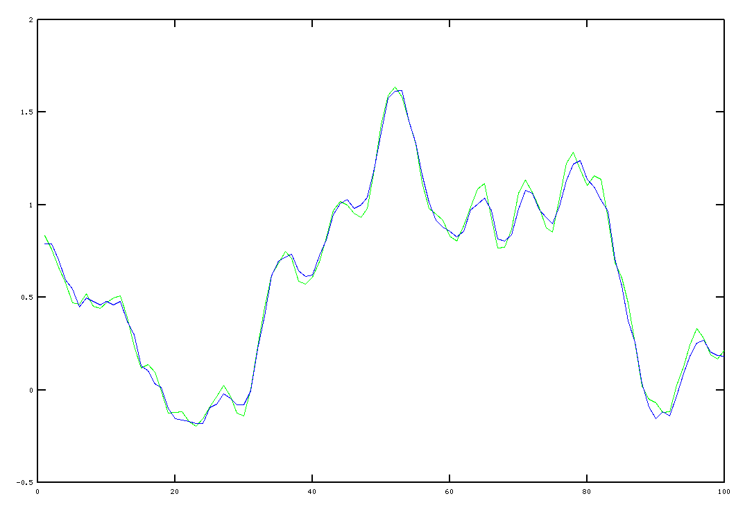
A simulation

To illustrate what is possible, here is a plot of an experimental fit. The green trace shows the original system's output sequence, while the blue trace shows the trajectory predicted by the model.

 

Some final comments

• I have found that, in practice, large levels of noise tend to produce models with poorly-scaled results. After building the model, you can try best-fitting a multiplier constant that scales all model terms to see if that improves the predictions. I don't have good theory to explain this...

• As the noise grows more significant with respect to signals, the best-fit models will start to become more random and less usable — partly an indication that there is not enough information to accurately distinguish signals and noise. You can try a much larger data set, or try pre-processing your raw measurements with filters to remove as much noise as possible before performing the analysis.

• This model is not in the right form to use with a classic Kalman filter. But it is a perfectly good ARMA model, and you already know how to transform an ARMA model^[4] into a model that does have the correct form. Right?

• And as for the extra outputs that you won't be able to observe? Don't observe them. Once your model has incorporated all of the extra information, the internal state updates operate the same way whether the extra variables are observed or not.

 

---

Footnotes: