Transition Matrix for Response Modes
Developing Models for Kalman Filters
Last time, an empirical analysis of correlation data gave an indication about what order of linear model might represent system behavior in a minimal but effective manner. However, in the process we determined some quantitative information as well. Is it enough to build a plausible state transition model?
A canonical model
We want a restricted form of model that is relatively simple to build, but still generic enough to represent a wide range of possible models. The particular structure that we will use is the following tridiagonal form.[1] This is the matrix structure obtained when applying a eigenvector transformation to a known state transition matrix. Notice that the parameter values in the lower left and upper right corners are all zero.
This fourth-order system is small enough to fit on the page, but big enough to illustrate the matrix structure and to represent the system order estimated in example of the previous installment.
This particular form has the following properties:
- The input can drive any of the next state equations. The
values of the
bparameters are set to either 1.0 or 0.0. - Every state can have a direct influence on the output, to be determined later by establishing parameter values in the observation equation.
- The only nonzero terms allowed in the state transition matrix are on the main diagonal and on the diagonals just above and below it. Many of the terms in the diagonals just above and just below the main diagonal can also be zero.
- The impulse response curves are hypothesized to be produced by separate states with minimal interaction.
- "The next value" for a state should be a lot like the value it had previously, otherwise the sampling interval was poorly chosen. This means that main diagonal terms will be positive, and reasonably close to 1.0 in value, but typically not exceeding 1.0 (which would be a warning of an unstable system).
Constructing the model
We will build up the model one or two lines at a time, at each step representing one of the long-term impulse response shapes observed during the correlation analysis.
exponential response
Suppose that a state variable has an initial value
x1. If the subsequent state variable values
are A x1, A2 x1,
A3 x1, and so forth, where A is a
positive number somewhat less than 1, this results in an exponentially
decaying pattern.
When undisturbed by additional outside influences after the first impulse, we can see that this same exponential behavior is generated using a one-state equation in the following form.
The critical parameter is the one that determines how much exponential
decay you get in how many time steps. The following chart shows values for
decay rate A necessary to result in a decay to half the
original value in N steps.
| Loge of attenuation per step | Steps for half-attenuation | A-value |
|---|---|---|
| -0.13863 | 5 | 0.87055 |
| -0.06932 | 10 | 0.93303 |
| -0.03466 | 20 | 0.96594 |
| -0.02311 | 30 | 0.977160 |
| -0.01733 | 40 | 0.982821 |
| -0.01386 | 50 | 0.986233 |
| -0.009242 | 75 | 0.990801 |
| -0.006932 | 100 | 0.993092 |
| -0.005545 | 125 | 0.9944701 |
| -0.004621 | 150 | 0.9953897 |
| -0.0039609 | 175 | 0.9960470 |
| -0.0034658 | 200 | 0.9965402 |
| -0.0027726 | 250 | 0.9972312 |
| -0.0023105 | 300 | 0.9976922 |
| -0.0017329 | 400 | 0.9982686 |
| -0.001386 | 500 | 0.9986147 |
| -0.0009242 | 750 | 0.9990762 |
| -0.0006932 | 1000 | 0.9993071 |
In the correlation analysis performed in the
previous installment, there were two exponential response patterns.
For the dominant pattern, the exponent was about -T/70 (or -0.01428 T),
which from the table above indicates that the model should
use a value of about 0.985. For the fast exponential,
the exponent was about -T/14 (or 0.07143 T). The table
indicates that the model should use a value of about 0.930.
exponentially decaying sine response
Modeling a sine wave involves two states. To see how to do this, start with the following proposed state transition equations.
Now simplify this a little. Assume that the model parameters
a11 and a22 are both
equal to 1.0. Assume that the
off diagonal terms a12 and a21
are equal in magnitude but opposite in sign, and much smaller.
Let the two b values be zero. Set the initial value
of x1 to 1.0 and x2 to
zero.
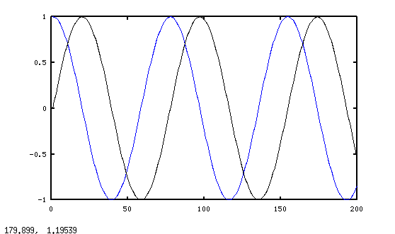
If we run a simulation of this sequence over a large number of steps, we get sequences of next-state values that looks like the following.
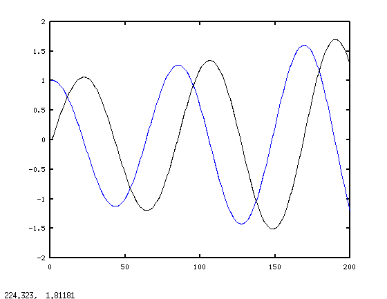
The two states produce results very much like a cosine and sine
functions, except for the unstable growth factor. If we scale every
term in the matrix times the factor 1.0 / sqrt( 1.0 +
a122 ) this stabilizes the oscillation.
As we have just seen, we can control the rate at which the sine waves decay away by adjusting the overall scaling of the four matrix terms. Using the exponential decay rates table as an inspiration, let's apply an additional scale factor on all matrix terms. For example, let's use the same factor that would reduce a simple exponential to half value in 75 steps.
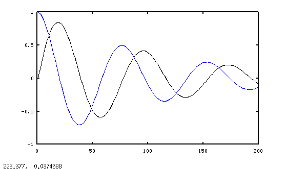
It certainly seems to have the desired effect!
It is pretty easy to tell what is happening to amplitudes at the peaks, but identifying a point on the wave attenuated to "half amplitude" somewhere between peaks is not so easy. For determining the decay multiplier to use, calculate the attenuation factor between consecutive peaks, and take the natural log of that. Divide that by the cycle length in samples. That gives you the attenuation per sample. You can look up this number in the leftmost column of the exponential attenuation table above, and then look in the column on the right to determine the multiplier value to use.
For the lightly damped sine wave identified in the correlation
analysis from the previous installment, we have already estimated that
the log of the attenuation rate is -1/700, or
-0.001429. Estimating from the lookup table, this
corresponds to about 490 samples for half-attenuation, close enough
to 500 samples that we can just use the entry for 500 samples directly:
0.9986.
The last remaining issue is adjusting the frequency, which is determined by the ratio of the on-diagonal and off-diagonal terms.
| Ratio | Period, samples |
|---|---|
| 0.004 | 1572 |
| 0.008 | 785 |
| 0.01 | 628 |
| 0.015 | 315 |
| 0.02 | 418 |
| 0.025 | 252 |
| 0.030 | 209 |
| 0.035 | 178 |
| 0.040 | 157 |
| 0.045 | 140 |
| 0.050 | 126 |
| 0.055 | 114 |
| 0.060 | 105 |
| 0.065 | 97 |
| 0.070 | 90 |
| 0.075 | 84 |
| 0.080 | 79 |
| 0.085 | 74 |
| 0.090 | 70 |
| 0.095 | 66 |
| 0.100 | 63 |
| 0.105 | 60 |
| 0.110 | 57.5 |
| 0.115 | 55 |
| 0.120 | 52.7 |
| 0.130 | 48.6 |
| 0.140 | 45.4 |
| 0.150 | 42.5 |
| 0.160 | 39.9 |
| 0.170 | 37.5 |
| 0.180 | 35.5 |
| 0.200 | 32.0 |
| 0.220 | 29.2 |
| 0.240 | 27.0 |
| 0.260 | 25.0 |
| 0.280 | 23.3 |
| 0.300 | 21.8 |
Applying this to the correlation analysis in the previous installment, we are looking for a period that is about 330 samples. Interpolating from the table above, the corresponding ratio to use is about 0.0148. This establishes the initial values of the off-diagonal terms. To adjust for the exponential attenuation, apply the scaling factor 0.9986 previously determined from the exponential decay table. Here are the results after the scaling.
We're most of the way there. We need to consolidate everything we know so far into a single state transition matrix, substituting values we have determined for coefficients.
Next time
We have set up a framework for representing the state transitions, but there is nothing yet to connect states to an output. If these states didn't happen to be driven by the same input sequence, there would be no relationship at all. We will continue next time to construct the model's output predictions.
Footnotes:
[1] See System Transformations, part 3 in this series.