Finishing the Correlation-Based Model

In the previous installment, we took the observations from an empirical correlation analysis to count the response modes related to model states, and constructed state equations that generate those patterns of response. This is what we have so far.

 

$$\begin{array}{c}{x_1}^{i+1}=0.985{x_1}^i+0.0{x_2}^i+0.0{x_3}^i+0.0{x_4}^i+1.0u^i\\ {x_2}^{i+1}=0.0{x_1}^i+0.930{x_2}^i+0.0{x_3}^i+0.0{x_4}^i+1.0u^i\\ {x_3}^{i+1}=0.0{x_1}^i+0.0{x_2}^i+0.9896{x_3}^i+-0.01477{x_3}^i+1.0u^i\\ {x_4}^{i+1}=0.0{x_1}^i+0.0{x_2}^i+0.01477{x_3}^i+0.9896{x_4}^i+0.0u^i\end{array}$$

 

However, we did not yet attempt to reconstruct the output sequence. We will do that this time, in the following steps.

1. Use the Octave system to apply the input data set from the correlation testing to the system state matrix, as constructed so far. Record the patterns of internal state variables generated.
2. Use Linear Least Squares methods to find the combination of those response patterns that best predicts the output sequence observed from actual system.
3. Use the best fit result to define the observation equation.
4. Check the results. Results are verified by running data through the system model equations a second time, comparing the final predictions to the actual system outputs.

 

The state expansion pass

We previously devised a state equation system to try. Read the input data sequence from the test data set. Start the state equations from an initial zero state, knowing no better information. Take the input values one at a time, apply them to the u input variable, and record what happens in the state vector x1 through x4. Place these values into a matrix by row; then each column of the matrix represents the trajectory of one state variable in response to the input sequence. Call this giant matrix X.

% Expand the response sequence of this state model
state = zeros(4,1);
Xstate = zeros(nrun,4);
for iterm=1:nrun
  Xstate(iterm,:) = state';
  state = Amat*state + Bmat*indat(iterm);
end

 

The output fitting pass

Octave makes this shockingly easy. If the state transition model were perfect, every output value will be predicted exactly by one specific combination of the generated state data. The combination takes care of all response-scaling issues. For the case of sine and cosine wave pairs, the relative weighting between the two establishes any required phase angle property.

Use the X matrix for the constraint matrix M of a linear least squares problem. This is the matrix of output patterns generated for each state variable. Use the vector of observed actual output values from the test input/output data set as the target Y vector for the Least Squares fit. Construct the normal equations and solve them.

MMat = Xstate'*Xstate;
RMat = Xstate'*outdat;
MInv = MMat^-1;
P = MInv*RMat;

Take the transpose of the best fit parameter vector P as the coefficients of the observation equation.

$$\begin{array}{c}{y}^i=c_1{x_1}^i+c_2{x_2}^i+c_3{x_3}^i+c_4{x_4}^i\end{array}$$

For reference, here are the observation equation coefficients produced by the best-fit calculations.

Cmat = [ 0.123202,  -0.149194, 0.047342, 0.027858 ]

 

The verification pass

We already know what the state variable responses are to the input sequence: this produces the matrix X. So, all that is left is to apply the "best fit" combination and generate the output prediction sequence.

yfit = Cmat * Xstate;

Here is a plot of the model predictions compared to the original system outputs as measured.

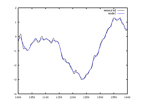
Perfect results are not expected. However, we can see that the overall performance is rather remarkable given the somewhat crude and subjective nature of the analysis used.

The most obvious discrepancies are an occasional fast oscillation, occurring sporadically. Remember that "high frequency glitch" that we chose to disregard in the correlation analysis? Well, here it is. It does appear to be more than a filtering artifact. But is it desirable? Not reproducing that particular behavior could be considered a beneficial result: an undesirable component of the response is eliminated by making the model simpler.

But on the other hand, we might now reconsider, and decide to add an additional response features to the model. The near-diagonal model structure is helpful for trying this, but we don't have any kind of reasonable parameter estimate. Next time we will revisit the LMS method and try "growing" a new impulse response mode.

 

---