LMS experiments

The LMS algorithm was introduced in this series as a means (very slowly) improve the values of parameters based on plentiful data. That would seem to apply in the situation of the model developed in a relatively subjective manner using correlation data. In our example study, we deliberately disregarded a fast oscillatory sort of disturbance in the correlation function, and perhaps that was a bad idea.

A feature of the "modal" state transition model is that it allows introduction of new states with a minimum of complication. Let's try using the LMS method to "grow" new states to account for the secondary behaviors that the previous model did not track well. Whether this is a good idea or a bad idea is up to you.

The problem

Start with the general discrete state model form.

\begin{matrix} {\overset{‸}{x}}^{i + 1} = A {\overset{‸}{x}}^{i} + B u^{i} \\ {\overset{‸}{y}}^{i + 1} = C {\overset{‸}{x}}^{i + 1} \end{matrix}

The parameters initially estimated for this model were as follows.

Amat =
   0.98900   0.00000   0.00000   0.00000   
   0.00000   0.93000   0.00000   0.00000   
   0.00000   0.00000   0.98960  -0.01477   
   0.00000   0.00000   0.01477   0.98960   

Bmat =
   1
   1
   1
   0

Cmat =
   0.12320  -0.14919   0.04734   0.02786

We can observe that the peculiar wobble decays to a a negligible level in 80 sample intervals or so, with an oscillating period of around 20 sample intervals. Based on this information, we can hypothesize an additional pair of states. Using the tables presented in a previous installment ^[1], initial estimates of new transition matrix parameters are selected. You can experiment with different initialization choices to see where they lead.

Two rows and two columns, initially filled with zero terms, are added into the state transition matrix. New initial values are then inserted along the main diagonal in the new rows.
Two new rows are added into the input coupling matrix. For the case of a state-pair, only one of the two terms needs to be driven by inputs, so one input coupling term is set to 1.0, the other to 0.0.
Two new observation terms are added into the output observation matrix. Since we never had these states before, the model currently does not observe the added states, and we set the two new observation parameters to initial values of 0.0.

Here is how the restructured model looks. A simulation can verify that the model produces the same results as before.

Amat =
   0.98900   0.00000   0.00000   0.00000   0.00000   0.00000
   0.00000   0.93000   0.00000   0.00000   0.00000   0.00000
   0.00000   0.00000   0.98960  -0.01477   0.00000   0.00000
   0.00000   0.00000   0.01477   0.98960   0.00000   0.00000
   0.00000   0.00000   0.00000   0.00000   0.92000  -0.30000
   0.00000   0.00000   0.00000   0.00000   0.30000   0.92000

Bmat =
   1
   1
   1
   0
   1
   0

Cmat =
   0.12320  -0.14919   0.04734   0.02786   0.00000   0.00000

Here are the Octave script lines to run the simulation to study the state updates, current output, and prediction error.

state = zeros(6,1);
for iterm=1:nrun
  out = Cmat * state;
  state = Amat*state + Bmat*indat(iterm);
  perr = out - outdat(iterm);
end

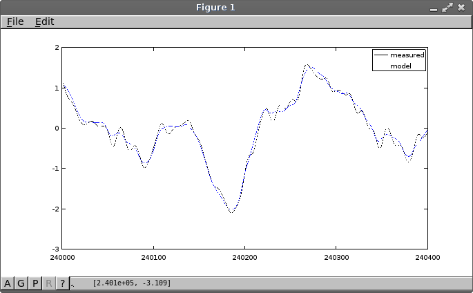
The following plot shows the initial simulation results before adjustments. This is exactly the same kind of response that we had previously with a four-state model, so no damage has been inflicted so far. Notice that the tracking is still plausible except when the extra oscillation becomes activated.

The adjustments

adjusting input coupling terms

The input coupling matrix B is not adjusted by these LMS updates. When using this form of decoupled model, each state is driven the same, independently, and the output observation terms account for all of the scaling.

adjusting observation matrix terms

The formula for the LMS updates to the output observation matrix is the following.

C \leftarrow \overset{‸}{C} - α Δ y x^{T} λ

We want to adjust only the output observation terms associated with the grafted new states, but the basic updating formula adjusts every observation term. To counter this, select the λ matrix to be a diagonal matrix with the values 1.0 in the last two columns corresponding to the new states, and with values 0.00 in all of the other main diagonal locations.

So these are the values to try for the observation equation updates.

alpha = 0.001;
lambda = [ ...
   0.00  0.00  0.00  0.00  0.00  0.00; ...
   0.00  0.00  0.00  0.00  0.00  0.00; ...
   0.00  0.00  0.00  0.00  0.00  0.00; ...
   0.00  0.00  0.00  0.00  0.00  0.00; ...
   0.00  0.00  0.00  0.00  1.00  0.00; ...
   0.00  0.00  0.00  0.00  0.00  1.00 ]

These are the LMS update calculations to apply.

  % Calculate the observation adjustment 
  delC = -alpha * perr * state' * lambda;
  Cmat = Cmat + delC;

adjusting the transition matrix

The basic LMS updating formula for the state transition matrix has a problem.

A \leftarrow \overset{‸}{A} - α Δ y C^{T} x^{T}

Because of the C term in the update equation, each matrix term is adjusted according to its influence on the output. But this means that states associated with new state terms will never change — making the whole exercise moot.

To counter this problem, set initial parameter values in the C matrix to 1.0e-6 instead of 0.0 so that these terms start negligibly small but do have a sign; then use the alternative update formula with sign(C) instead of C in the update equation.

There is another problem. The updates could potentially affect all matrix terms, but we only want the adjustments to be applied to the terms that are in the rows and columns for the new states.

One way to force these adjustments is to apply the same λ matrix used with the observation updates. The following updating formula takes all of the special adjustments into account.

A \leftarrow \overset{‸}{A} - α Δ y λ {sign(C)}^{T} x^{T} λ

Here are the calculations to apply during the simulation, including the special tweaks.

  alpha = 0.00002;

  % Calculate the transition matrix adjustment 
  Csign = sign(Cmat);
  delA = -alpha * perr * lambda * Csign' * state' * lambda;
  Amat = Amat + delA;

Letting it work

Insert the additional calculations into the simulation loop, where the incremental changes to the observation matrix and state transition matrix are applied.

Let's throw the switch and see what happens in the modified simulation.

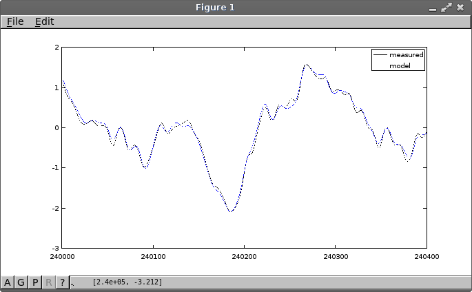
This takes a long time to run. A very long time. The adjusted tracking is still not perfect, but a lot better at following the high frequency wobbles. After 250000 LMS adjustments, there are some small improvements and the "wobbles" are tracked somewhat more closely. Here is the new simulation result.

Here are the adjusted parameter estimates at the end of training.

Cmat =
   0.1232020  -0.1491940   0.0473420   0.0278580  -0.0145235   0.0036879

Amat =
   0.98900   0.00000   0.00000   0.00000   0.00000   0.00000
   0.00000   0.93000   0.00000   0.00000   0.00000   0.00000
   0.00000   0.00000   0.98960  -0.01477   0.00000   0.00000
   0.00000   0.00000   0.01477   0.98960   0.00000   0.00000
   0.00000   0.00000   0.00000   0.00000   0.92395  -0.29938
   0.00000   0.00000   0.00000   0.00000   0.29541   0.92115

The success of this experiment must be considered mixed. As we have seen, the LMS approach is relatively simple when allowed to tune everything, but the adjustments to tune some things but not touch others can become somewhat complicated. The extra "wobble" response is probably coupled more to some kind of internal noise source and only weakly correlated to the input signal. No model adjustments could fully predict that behavior.

Variants

Some alternative strategies that could be explored are:

Try tuning the new response parameters as an independent LMS problem, and then merge them into the combined state transition matrix later.
Let the LMS adjustments have free run to adjust any of the state transition parameters, then go back and restructure the equations afterwards.
Forget the structure. Just use whatever adjustments the LMS algorithm comes up with for all matrix terms.

For next time

In this installment, we tried some experiments with growing state transition equations. We started with a model that was in a highly diagonal form. But that is not in general a requirement. You can append additional states to a state transition model with any sort of structure. You can tune new states separately, or all states together. The LMS method doesn't care.

This kind of adjustment is appropriate when you think that something is missing from your existing model. But suppose that the state equations are suspected of being more complicated than they need to be. Is there a way to shrink them?

Footnotes:

[1] See Transition Matrix for Response Modes in this series.

LMS: Experiments in Tuning New States