Generating Correlated Random Vectors
Developing Models for Kalman Filters
For purposes of studying our noise models, we want to be able to exercise our state transition equations with noise sources that have known covariance properties. In this installment, we will discuss a way to simulate the correlated noise sources.
The Choleski factorization
Variance matrices have a symmetry property, Q = QT.
This is because each covariance matrix term Qi,j
results from averaging pairs of terms xi · xj, which are always equal to the
commuted product terms xj · xi. The main diagonal terms of a covariance matrix result from
products of one random term with itself, yielding a sum of squared values, so it is never negative. Excluding pathological cases, all of the main diagonal terms of the covariance matrix will be positive and will dominate the off-diagonal terms, which could be of either sign.
What is a little less obvious is that covariance matrices (and other matrices
like them) can be factored into "square root" matrix forms. That is, for any such
(symmetric, real-valued, positive definite) matrix Q, it is possible
to find a matrix factor q such that
Q = q qT
In fact, an infinite number of such factorizations are possible. To show this,
suppose that you already know of one factorization Q = q qT . We can note that any orthonormal matrix U will have the
property that its transpose is its own inverse. Consequently:
( q U ) ( q U ) T = ( q U ) ( UT qT ) = q qT
So if q is a factor matrix, ( q U ) will be a
similar sort of "square root" matrix also.
But there is one particular factorization that is computationally very useful:
the one for which the q matrix is lower triangular. This one
is easy to determine, and easy to use.
Finding triangular factors
Let's step through a factorization of a symmetric 3x3 covariance matrix
X. Once you see the pattern, you can extend this to any order matrix.
If you are a purist, you are welcome to construct a formal proof by integer
induction.
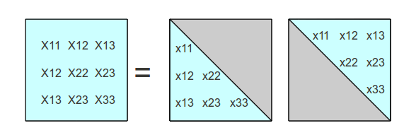
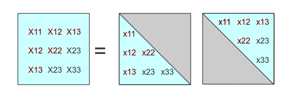
We start with the factored form that we want to find. We know the terms of
the X covariance matrix. When we finish, we want to know the
terms in factor matrix x, with its corresponding transpose.
As shown in the following illustration, the grayed-out terms are all equal to
zero and are of no consequence.
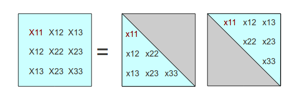
We first observe that the X1,1 term results from the
dot product of the first row of factor matrix x with the first column of
its transpose, which turns out to be the same vector terms but with the terms in
a different orientation. Since only the first term of the vectors is non-zero,
this dot product is relatively trivial. We can determine immediately that the factor
matrix must satisfy the condition
X 1,1 = x1,1 * x1,1
→ x1,1 = √ X1,1
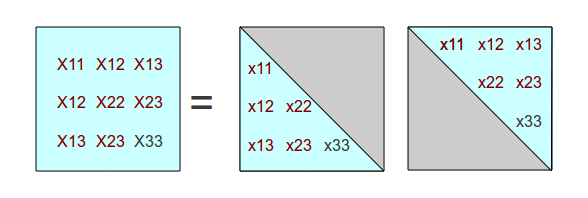
We can color highlight in red the terms that have been processed and that have known values.
If we now consider work downwards and consider the next two terms in the
first column of the X matrix, these terms must be formed by dot
products between the other two rows and of the factor matrix and the known
first column of the transposed matrix (which happens to have only one non-zero
term). These dot products also involve only one multiplication each, and
the following conditions must hold.
X1,2 = x1,2 * x1,1
X1,3 = x1,3 * x1,1
Knowing the value of x1,1 it quickly follows that
x1,2 = X1,2 / x1,1
x1,3 = X1,3 / x1,1
So far, we have the following processed terms.
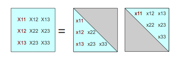
But when we take advantage of the fact that the second factor matrix will be the transpose of the first one, some additional terms are known and need not be calculated again.
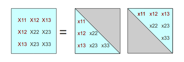
Now we can start working down the second column of the X covariance
matrix. The X2,2 term results from the product of the
second row of the factor matrix with its transpose, so the following conditions must
be satisfied.
X2,2 = x1,2 * x1,2 * x2,2 * x2,2
We already know the value of x1,2 , so we quickly
determine that
x2,2 = √ ( X2,2 - x1,2 * x1,2)
Working the way down the rest of the second column, we must satisfy
X2,3 = x1,2 * x1,3 + x2,2 * x2,3
Knowing the values of x1,2 and x1,3, we can calculate
x2,3 = ( X2,3 - x1,2 * x1,3) / x2,2)
Again taking advantage of the symmetry, and reviewing how many terms remain, we find that only one unknown term remains.
For this term, we can determine that it must satisfy the condition
X3,3 = x1,3 * x1,3 + x2,3 * x2,3 + x3,3 * x3,3
x3,3 = √ ( X3,3 - x1,3 * x1,3 - x2,3 * x2,3)
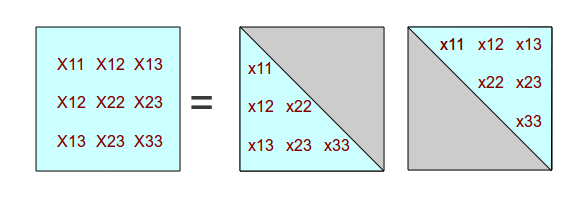
The factorization is now done. To verify, calculate the product of the two triangular factors and check that the result reproduces the original covariance matrix.
Once you are completely comfortable with the Choleski decomposition,
you can forget about all of the internal details, and simply let
the Octave / Matlab chol command to do all of these matrix
calculations for you.
A quick example
Define a real-valued, symmetric initial matrix.
Qmat =
   1.0000000   0.8100000   1.0000000   0.0100000
   0.8100000   0.7186000   0.7475000   0.0706000
   1.0000000   0.7475000   1.0664062  -0.0018750
   0.0100000   0.0706000  -0.0018750   1.7187000
Apply the chol command to produce the upper and lower
symmetric triangular factors.
f2 = chol(Qmat)
f1 = f2'

f1 =
   1.00000   0.00000   0.00000   0.00000
   0.81000   0.25000   0.00000   0.00000
   1.00000  -0.25000   0.06250   0.00000
   0.01000   0.25000   0.81000   1.00000

f2 =
   1.00000   0.81000   1.00000   0.01000
   0.00000   0.25000  -0.25000   0.25000
   0.00000   0.00000   0.06250   0.81000
   0.00000   0.00000   0.00000   1.00000
Multiply the two factors together again and compare to the original symmetric matrix to see if they match within statistical tolerances.
restored = f1 * f2

restored =
   1.0000000   0.8100000   1.0000000   0.0100000
   0.8100000   0.7186000   0.7475000   0.0706000
   1.0000000   0.7475000   1.0664062  -0.0018750
   0.0100000   0.0706000  -0.0018750   1.7187000
Yes, but what good is this?
For right now, here is the particular application we care about. Suppose that you
start with three statistically independent streams of random values with zero
mean and variance 1.0, collected to form a column vector
x. As you know from past articles, when a huge number of
the rank-one matrix products x xT are averaged,
the results will converge to a covariance matrix. Since each random term
is independent from the others, this matrix converges to an identity
matrix.
So now, suppose that the desired covariance matrix is Q. Compute
its Choleski factorization q qT.
Q = q qT
Now take the same set of random vectors x as before, and transform
them by calculating the matrix-vector product q x.
Observe that the rank-one product terms using these vectors will look
like the following.
(q x) (q x)T = q x xT qT = (q) (x xT) (qT)
Now average a huge number of these products to obtain the expected
value. The outer q terms are just constant multipliers,
so this converges to
      q E( x xT) qT  =

      q I qT  =

      q qT  =

      Q
And there you go! You can now take a set of independent, uncorrelated random variables and combine them in such a way that you get a new set of random variables showing the noise correlation properties you want.
A demonstration
Let's build some random vectors and verify that this works. Generate vectors of independent, normally-distributed random vectors with variance 1.0. Apply the Choleski matrix to each vector, and then calculate the estimated covariance matrix using rank-one updates. Then let's see if the covariance estimate is the one we wanted.
% Script to verify correlation in a generated random sequence.

% Define desired correlation matrix and its factors
Qmat = [
   0.1000000   0.0800000   0.0000000   0.0100000;
   0.0800000   0.7186000   0.0275000   0.0000000;
   0.0000000   0.0275000   0.0964062  -0.0018750;
   0.0100000   0.0000000  -0.0018750   0.2564062 ]
 qfact2 = chol(Qmat);
 qfact1 = qfact2'

 estm = zeros(4,4);
 for term=1:250000
   vect= qfact1 * randn(4,1);
   estm = estm + vect*vect';
 end
 estm = (1/25000)*estm
estm =
   1.0005e+00   8.1153e-01   2.5921e-04   1.0314e-01
   8.1153e-01   7.1906e+00   2.6385e-01   5.8694e-04
   2.5921e-04   2.6385e-01   9.6338e-01  -1.7193e-02
   1.0314e-01   5.8694e-04  -1.7193e-02   2.5680e+00
Next time, we will apply this to the study of covariance propagation in state transition equations.