Noisy Observer Simulation

For purposes of studying observer models and their response to noise, we want to be able to exercise the model equations with noise having known covariance properties. The benefits of this are that we can verify that the noisy models behave reasonably like the actual system, and we can also study the effectiveness of observer gains.

Last time, we showed how to set up correlated noise generators producing random vectors with any suitable correlation. Now we will apply this, and take a look at the kind of responses to expect from the observer.

Simulating the noisy system

Start with the state transition equations in the usual form. The output of the system is a direct readout of one of the states, making it relatively easy to see how good an observer is doing at tracking that state.

% Construct the state model 
Amat = [ ...
   1.03,  0.14,  0.0,    0.0 ;  ...
  -0.10,  0.92, -0.09,   0.0 ;  ...
   0.0,   0.20,  0.88,  -0.40;  ...
   0.0,   0.0,   0.00,   0.78;   ];
Bmat = [0, 0, 0, 1.00 ]';
Cmat = [1.00, 0.00, 0.00, 0.00 ];

For purposes of studying the noise response, set the input coupling matrix B to zero — or equivalently, simply omit the input driving terms temporarily.

Establish the noise covariance matrices Q for the state noise source and R for the observation noise source. Use the Choleski decomposition to determine the "square root" triangular factors q and r for these matrices. For the special case of one output variable, specify the square root of the observation noise variance.

% Random noise correlation matrices
Wmat = [ 0.04,  0.01, -0.01, 0.00; ...
         0.01,  0.025, 0.01, 0.00; ...
        -0.01,  0.01,  0.25, 0.02; ...
         0.00,  0.00,  0.02, 0.05; ];
Vmat =  0.016;

% Factor covariance matrices for generators
wtri = (chol(Wmat))';
vtri = (chol(Vmat))';

It is now possible to run a correlated noise simulation for "noise only" effects.

% Reserve storage for the real system simulation from random state
stateN = (rand(4,1)-0.5*ones(4,1))*2.0;
XstateN = stateN';
YoutN = zeros(nrun,1);
outN  = Cmat*stateN;

% Run simulation
for iterm=1:nrun
  % Noisy system simulation, next noise terms
  noiseX = wtri * randn(4,1);
  noiseY = vtri * randn;

  % Noisy system simulation, next state
  XstateN(iterm,:) = stateN';
  YoutN(iterm) = outN;
  stateN = Amat*stateN + noiseX;
  outN = Cmat*stateN + noiseY;
end

To test state observer equations against this simulated system, run the observer calculations in parallel.

% Reserve storage for the observer system from zero state
stateO = zeros(4,1);
outO  = 0.0;
XstateO = zeros(nrun,4);
YoutO = zeros(nrun,1);

% Run state observer
for iterm=1:nrun
  % Observer projection step
  XstateO(iterm,:) = stateO';
  YoutO(iterm) = outO;
  stateO = Amat*stateO;

  % Observer correction
  outO = Cmat*stateO;
  Xcorr = Kmat * (outO-outN);
  stateO = stateO - Xcorr;
end

Let's see how the two compare using the following observer design.

% Construct the observer gains
Kmat = [  0.075  0.35  0.55  0.17 ]'

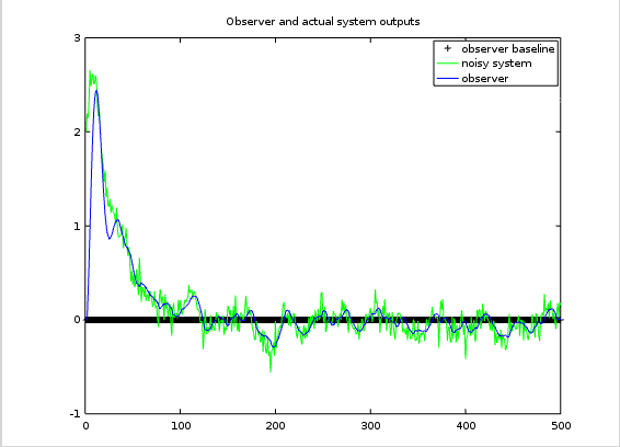
Some things to notice about this particular plot:

With observer gains of zero and no driving input signal, there is nothing to displace the observer output from a "flat line" at zero. That is the "quiescent state."
The initial state uncertainty starts very large. If you have no better information, there is nothing that can be done about this. A bit transient is unavoidable.
About 100 sample intervals are required for the initial state displacement effects to settle away completely. This is a property of the system's transient response.
The state observer is able to bring its state estimates into proximity of the noise-disturbed system state in about 60 sampling intervals. This depends primarily on the observer settling characteristic.

This is an ordinary state observer, for the case in which noise signals are stationary and the linear model is time invariant. This covers a lot of territory, but it still isn't a Kalman Filter. So, what can the Kalman Filter add to this? Two things:

if you have a very complex system with precisely known changes in the state transition matrix and in the noise variance properties at every time instant, the Kalman Filter can adjust to the specified new conditions.
the Kalman Filter state estimates will converge to track the transient conditions more quickly in the initial start-up.

Those considerations could be important, or they could be irrelevant. So consider carefully what your requirements are.

Next time, we will take a closer look at a systematic approach to selecting the observer gains.

[1]

Simulating the Noisy Observer

Simulating the noisy system