Consistent Covariances

A major hole in the Kalman Filter story remains. Kalman Filtering assumes that all of the model parameters are known perfectly. That includes all of the covariance noise model terms.

Let's quickly review the state of the art for determining the internal covariance models. Assume that the covariance matrices are diagonal. Any questions?^[1]

Understanding the Kalman Gains

Let's think about the optimal Kalman Gains equations for a moment, in particular, the steady-state Kalman gains. As we have seen in preceding installments, the optimal gain is determined from these equations:

To consider what is going on here, suppose that the equations are for an order 1 system, so that the covariance matrices reduce to scalars. With a little elementary algebra, the Kalman optimality conditions reduce to the following expression.

             a2 p c + w c
  K = ---------------------------
         a2 c2 p + c2 w + v

Without loss of generality, further presume that the observation of the output is done with an observation gain c equals 1 so that it can be disregarded.

           a2 p + w
  K = ------------------------
         a2 p + w + v

Furthermore, the state transition term is not very different from 1.0, so use that value as an approximation.

            p + w
  K ≈   --------------
          p + w + v

Now lets consider a some extreme cases.

• The model has negligible internal noise w and observation noise dominates. The Kalman gain gets very small. Consequently p gets very small, and the numerator in the expression for K gets very small. In other words, if the noise has nothing to do with the states, the optimal strategy is to not allow noise to reach the states through the Kalman gain feedback. Use minimal corrections — let the state transition model run unadjusted as the observer.

• The model has insignificant observation noise v. The optimal Kalman gain value approaches 1.0. That is, the optimal strategy is to expend maximum effort to try to make the state consistent with the observed output quickly.

• Any situation between these extremes is a balancing act. Which can you trust more, the state estimates initially produced by the initial model projection, or corrections indicated by the measured outputs? If the measurement noise dominates, make lesser adjustments to the state variables. If the internal state noise dominates, make larger corrections to the state variables.

A somewhat unexpected consequence of this is that the absolute values of the variances don't make much difference to the determination of the Kalman gains. The relative sizes of the variances is what makes the most difference. However, the absolute sizes make a big difference to simulations of noisy system response.

Properties of observed noise

The noise can be considered to consist of two parts.

1. The noise generated in the measurement channels independent of the system state.
2. Correlated noise generated in the states by propagation of state noise and feedback influences over time.

There are some assumptions that you can reasonably make about the measurement noise. (And you can independently test these assumptions to verify them.)

• Measurement channels that are adequately isolated will not not exhibit significant "crosstalk" coupling to correlate measurements between channels.
• Measurement channels that are adequately shielded will not not pick up seemingly simultaneous noise excitation from interfering noise sources.
• Measurement channels are designed for low noise and do not have significant "common mode" spurious noise signals.
• Transient responses, if they should occur, are so fast that they appear virtually the same as "impulse noise," and thus all frequencies are expected to be disturbed equally.
• Signal sensors on different channels operate independently.

It is therefore reasonable to assume that the measurement noise is independent in each of the measurement channels, with no covariance of any relevance between channels, and nothing to limit the frequency band exhibited by this noise. The covariance matrix V for measurement noise is diagonal and positive definite. White noise is a reasonable representation.

You can obtain an FFT of your system response by a process something like the following. (Notice that you can't average FFT's directly, because the random phase of the frequencies will cancellations that tend to drive all of the terms toward zero. However, you can average the absolute values or the power spectral densities and obtain meaningful results.)

Now, suppose that your system is driven by a random signal. Take arbitrary blocks of output signal data and apply an FFT analysis in the following manner.

for iblock=1:reps
   % Read block of 1000 output samples into "outdat" array
   spect = fft(outdat);
   spsum = spsum + abs(spect);
end
spsum = spsum / reps;

plot(1:501,spsum(1:501),'b')
title('FFT of output response data')

In the plot, location 500 corresponds to the Nyquist limit for the sampling rate.

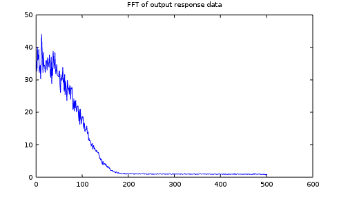
That "flat line" portion of the line that extends through the full band is the result of the "white noise". The "peaks" at lower frequencies are the effects of correlation on top of the "white noise" floor. By getting rid of the lower frequencies, it is possible to distinguish the measurement noise effects. That can be done by filtering the raw output measurement data.

Construct the following function in Octave and save it to the file hfpilt.m where Octave can find it.

function [outpt,newstate] = hpfilt(inpt,oldstate)
% Function to calculate next value of white noise isolation filter
bcoeff = [ 0.072192  -0.325628   0.619465  -0.619465   0.325628  -0.072192 ];
acoeff = [ 1.0000000  -0.1992412   0.6783060  -0.0867833   0.0670991  -0.0031408 ];
outsum = bcoeff(1)*inpt;
outsum = outsum + bcoeff(2:6)*oldstate(1:5);
outpt  = outsum - acoeff(2:6)*oldstate(6:10);
newstate = [0.0; oldstate(1:9)];
newstate(6) = outpt;
newstate(1) = inpt;
return; 

To use this to filter data, pass the original data stream through one value at a time and save the results.

hpstate = zeros(10,1);
filtdat = zeros(1,nrun);
for  iterm=1:nrun
  [newout,newstate] = hpfilt(outvalue(iterm),hpstate);
  filtdat(iterm) = newout;
  hpstate = newstate;
end

Here is an example of the spectrum plot for the filtered data stream. Notice the dramatically different scaling on this plot. Low frequencies have been reduced to virtually nothing.

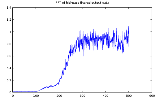
Now it is a simple matter calculate the variance (mean sum of squared values) for the filtered data stream. The value you should use for the variance of the measured signal channel in your model is twice that number — because the filtering removed the half of the broadband white noise energy that was in the lower half of the spectrum, along with the correlated noise.

Consistent state variance terms

The second part of the variance mystery is the noise being applied to the hidden model state variables. In general, it is not possible to determine exactly what these noise effects are.^[1] However, it is possible to establish some sort of state noise variance model that is at least consistent with the observer gains, the channel noise model, and what is observed in the output data.

Here is an ad-hoc relaxation algorithm that you can use to do this.

1. Start with reasonably good estimates for the observation noise covariance matrix V.

2. Use any method that you like to select reasonably good observer gains for your system. They don't need to be optimal.

3. Obtain real system data, using small randomized signals. You don't want the system "stuck" in an extremely tiny range, but you don't want the results to be overpowered by a very large drive signal. Apply the randomized input sequence to the system and observe the output.

4. Calculate the observer output sequence using known signal data and observer gains.

5. Calculate the (co)variance Y for the difference between the actual outputs and the model predictions.^[2]

6. Precalculate some intermediate terms.

       M  =  [I - K C] A  
   
       N  =  K V KT
   
       G  =  CT (C CT)-1 
   

7. Initialize the Q, P, and X matrices to zero.

8. Select a relaxation multiplier α, positive and less than 1.0, perhaps 0.02 to 0.10.

9. Iteratively apply the variance propagation equations in the following sequence.

   D  =  (Y - X)
   Q  ←  Q + α G D GT
   P  ←  M P MT + N + Q
   X  =  C P CT + V  
   

10. Continue the iterations until the adjustments to the Q matrix become negligible. All that this is doing is tracking the variance propagation through the system to simulate the sample-by-sample updates. If the difference between the estimated observer variance X and the actual tracking error Y becomes negligible, whatever the value of the Q matrix is at that point becomes the state noise variance estimate — close enough. Otherwise, the Q matrix is adjusted in a manner that should push future variance predictions in the right direction.

 Q  = Q + α G D GT
    = Q + α CT (C CT)-1 D (C CT)-1 C 

  X = ...  +  α C CT (C CT)-1 D (C CT)-1 C CT 

  ... +  α D 

  D = Y - X - α D
      = (Y - X) - α (Y-X) 

It's not much, but let's call this "the state of the art in applied guesswork."