The Dreaded Kalman Divergence

Imagine an application in which the usual assumption of a stable system is stretched — for example a satellite navigation problem. You know that in a couple of centuries its orbit is going to decay and the satellite will come a-crashing down. But for all practical purposes, once you set the thing in motion, it stays in motion. It does not settle gently and asymptotically back to earth while you watch.

Or suppose that information available for building the model is limited, and in an attempt to make up for that, there are numerous unverified (unverifiable?) structural assumptions deeply embedded in the state transition model. If not corrected, errors resulting from the questionable assumptions can persist and accumulate over very long periods of time.

Suppose further that the variance models assumed for this system are fundamentally flawed. Meaningful cross-correlation dependencies are assumed away. The Kalman model, as we have seen, tends to trust the model estimates for internal states that it can't observe directly — consequently, the Kalman corrections can leave some important internal state variables essentially untouched.

A Kalman Filter model is set up under these assumptions and conditions. A state with large initial uncertainty is assumed. The Kalman filter seems to work great!

But shortly thereafter the hammer falls. Creeping trajectory errors appear. The predictions of the observer gradually diverge from the actual system behavior, eventually deviating so badly that the results are useless. Welcome to the dreaded Kalman Divergence Problem.

 

An example

Let's take a very simple two-state case. The system is marginally stable. Changes in velocity are driven randomly. The velocity is then integrated to determine the current position. The random input sequence is zero mean, so the deviations affecting the velocity are balanced. Unless something is done to accelerate this system deliberately, the velocity should remain centered around its initial zero value forever.

But it doesn't happen. Here is a typical example of what occurs. This is known as a "random walk."

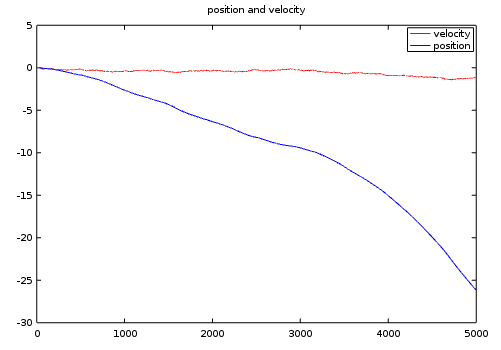
Not only can the position state diverge away to infinity, so can the velocity variable. This effect is well known, oft forgotten, and worth remembering:

In other words, the system could end up anywhere, given enough time. If the Kalman Filter system formulation does not observe or respond to this drift, you're in deep trouble.

 

The state of the art

Amidst the wailing and gnashing of teeth, you might hear cries, "But I am updating the covariance equations according to the textbooks, very carefully, so variance estimates should adapt over time to correct the problem." Of course, as a careful reader of this series, you will know that the covariance updates don't adapt to anything. They are based solely on assumptions hard-coded into the covariance and transition model matrices. If those assumptions, however plausible, lead to a bad result, maybe it would be a good idea to fix the assumptions?

In other words, the problems occur because the transition model is deficient, the variance models are mostly fictional, the observation is incomplete. Then the Kalman Filters are are expected to optimize all the problems away. Is that wishful thinking or what? An IEEE reprint series^[1] has a whole section of papers devoted to quantifying the impact of model deficiencies, and how they lead to tracking difficulty. But there isn't a whole lot of ready advice regarding remedies.

The fact that the Kalman filter equations can behave quite rationally at first suggests that estimates of the P state covariance are considerably lower than they should be. One cute solution ^[2] proposes artificially pumping up the P internal state variance estimates before applying the variance updates. This is a first cousin to the forgetting factors we mentioned in passing when discussing adaptive systems. This scheme applies a small positive inflation factor α to enlarge the state variance matrix at each update step. Following that, the covariance propagation equations are updated in the ordinary way.

$$P\leftarrow P·\left(1+\alpha \right)$$ $$W\iff \left(AP{A}^T+Q\right)$$ $$X\iff \left(CW{C}^T+V\right)$$ $$P_{i+1}=W+KCW+W{C}^T{K}^T+KX{K}^T$$

What you see is what you get. Things often "seem better." Maybe anything is preferable to going unstable. Still, it is hard to say how this kind of fixup has any relationship to the the supposedly optimal performance. Optimizing what exactly?

 

Alternative solutions?

It is worth noting that the humble alpha-beta filter is invulnerable to problems of this sort, because anomalous behaviors would be adjusted away by the manual tuning of the gain parameters.

Having reached this point in the series, you are no longer entirely reliant on the Kalman gain equations to determine your observer gains. You know how to simulate your system and test your selected gains. You can calculate the steady-state Kalman gains that result from your modeling assumption. Starting from there, you can manually adjust steady-state gain parameters until the Kalman Filter is no longer subject to divergence anomalies. Tweaking the Kalman gains is likely to provide an inexpensive but effective fix.

Another idea is to apply a relaxation algorithm, such as the one covered in the previous installment, to suggest a variance model that is more consistent with the state transition model structure. This idea might be extended for adapting the variance model to changing conditions, but these calculations do not come cheap.

As you know, it is not necessary to always use Kalman gains exactly as calculated. You could determine constant, non-optimal observer gains that have good global stability properties. Then, the gains you actually apply for the observer can be a suitable mix of Kalman optimal gains with a small amount of stabilizing gains.

 

---